Quick Start

This section provides an introduction to using PetroFit. It also highlights essential functions in conjunction with Photutils and Astropy. For in-depth explanations, refer to the respective sections of interest within this documentation.

To start with PetroFit, simply import it as follows:

import petrofit as pf

Loading Example Data

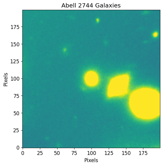
The following data is a cutout of a group of bright galaxies in Abell 2744 (located at (3.596248, -30.388517)). The original data was acquired by the Hubble Frontier Fields team via the WFC3 instrument in the F105W filter and can be directly downloaded from the Mikulski Archive for Space Telescopes. The cutout image used in this documentation can be found in the git repository at the following path petrofit/docs/data/abell_2744_dwarf_galaxy_f105w.fits.gz.

Loading Image

You can use astropy’s CCDData to load the example data and visualize it through matplotlib. Note that CCDData.read does not return a 2D array, but rather a CCDData instance which contains the image array, header, and WCS. To access the image array stored in the CCDData use the data attribute (i.e. CCDData.data as shown in the plt.imshow command below).

from astropy.nddata import CCDData

image = CCDData.read('data/abell_2744_dwarf_galaxy_f105w.fits.gz')

import numpy as np
from matplotlib import pyplot as plt

plt.rcParams['figure.figsize'] = [6, 6]
plt.rcParams['image.origin'] = 'lower'
plt.rcParams['font.size'] = 12

vmax = 0.05 # vmax for matplotlib imshow
vmin = - vmax

plt.imshow(image.data, vmin=vmin, vmax=vmax)
plt.title("Abell 2744 Galaxies")
plt.xlabel("Pixels")
plt.ylabel("Pixels")
plt.show()

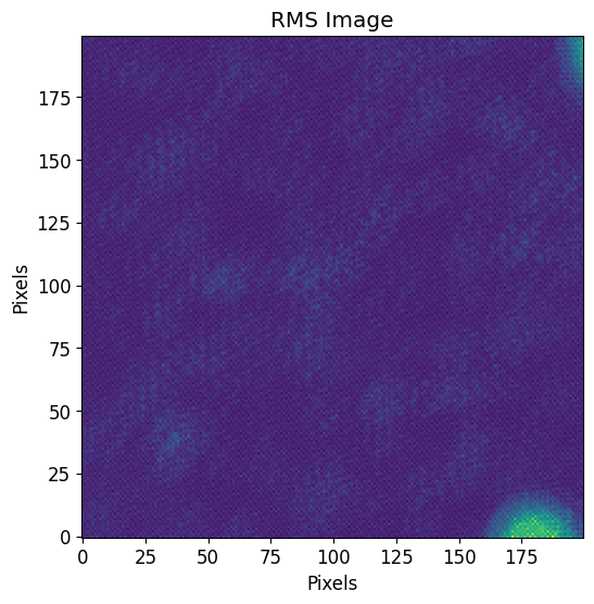
Loading RMS Image

Since we only want the rms image array, we use astropy’s io.fits.getdata function as follows:

from astropy.io import fits
rms = fits.getdata('data/abell_2744_dwarf_galaxy_f105w_rms.fits.gz')

plt.imshow(rms)
plt.title("RMS Image")
plt.xlabel("Pixels")
plt.ylabel("Pixels")
plt.show()

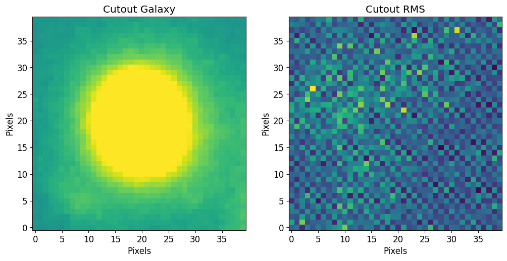
Making Cutouts

You can use astropy’s Cutout2D function to make cutouts of sources. To access the data (image array), use the data attribute (i.e. Cutout2D.data as shown in the plt.imshow command below). Note that position can be a SkyCoord if you provide the Cutout2D function a WCS.

from astropy.nddata import Cutout2D

# Make cutout image, centerd at (100, 100) pixels, 40 pixels in size
cutout_image = Cutout2D(image, position=(100,100), size=40)

# Make cutout rms, centerd at (100, 100) pixels, 40 pixels in size
cutout_rms = Cutout2D(rms, position=(100,100), size=40)

# Plot cutouts
# ------------
fig, axs = plt.subplots(1,2, figsize=(12, 6))

plt.sca(axs[0])
plt.imshow(cutout_image.data, vmin=vmin, vmax=vmax)
plt.title("Cutout Galaxy")
plt.xlabel("Pixels")
plt.ylabel("Pixels")

plt.sca(axs[1])
plt.imshow(cutout_rms.data)
plt.title("Cutout RMS")
plt.xlabel("Pixels")
plt.ylabel("Pixels")
plt.show()

Defining AstroPy Sérsic Models

This example shows how to define a 2D Sérsic model using astropy. We fill in our initial guess for the parameters (or correct parameters if we know them) when initializing the Sersic2D object.

To assist users, PetroFit offers a function named get_default_sersic_bounds that provides a default set of bounds for the Sérsic model parameters. This function is particularly useful when you’re fitting data as these bounds help in constraining the fitting parameter space.

The dictionary returned by get_default_sersic_bounds has parameter names as its keys. The values are tuples where the first element indicates the minimum allowed value and the second element indicates the maximum. In situations where there’s no constraint on a parameter’s value, None is used.

For instance, the dictionary looks like this:

# get_default_sersic_bounds returns:
bounds = {
    'amplitude': (0., None),
    'r_eff': (0, None),
    'n': (0, 10),
    'ellip': (0, 1),
    'theta': (-2 * np.pi, 2 * np.pi),
}

from astropy.modeling import models

sersic_model = models.Sersic2D(

        amplitude=10, # Intensity at r_eff
        r_eff=1, # Effective or half-lilght radius
        n=4, # Sersic index
        x_0=20, # center of model in the x direction
        y_0=20, # center of model in the y direction
        ellip=0.1, # Ellipticity
        theta=0.0, # Rotation angle in radians, counterclockwise from the positive x-axis.

        bounds=pf.get_default_sersic_bounds(), # PetroFit parameter bounds
)

To add x_0 and y_0 bounds to the default bounds, you can update the dictionary as you would a regular Python dictionary. You can add or update bounds by passing a Python dictionary to the get_default_sersic_bounds function as follows:

bound_dict = pf.get_default_sersic_bounds({
    'x_0': (10, 30),
    'y_0': (10, 30)})
bound_dict

{'amplitude': (0.0, None),
 'r_eff': (0.001, None),
 'n': (0.1, 10),
 'ellip': (0, 0.99),
 'theta': (-6.283185307179586, 6.283185307179586),
 'x_0': (10, 30),
 'y_0': (10, 30)}

You can also directly update the model bounds as follows:

sersic_model.bounds.update({'x_0': (10, 30),  'y_0': (10, 30)})

Making Compound Models (Combining Models)

You can combine multiple models to form a compound model by adding, subtracting, multiplying, and dividing individual models. For example, we add the Sérsic model from the last section to itself to form a two-component Sérsic model (notice that the number of parameters double):

compound_sersic_model = sersic_model + sersic_model

pf.print_model_params(compound_sersic_model)

10.0000 amplitude_0
1.0000  r_eff_0
4.0000  n_0
20.0000 x_0_0
20.0000 y_0_0
0.1000  ellip_0
0.0000  theta_0
10.0000 amplitude_1
1.0000  r_eff_1
4.0000  n_1
20.0000 x_0_1
20.0000 y_0_1
0.1000  ellip_1
0.0000  theta_1

Making a PSF Convolved Model

PSFConvolvedModel2D is an extension of Fittable2DModel designed to incorporate PSF convolution and facilitate image sampling for models native to astropy. This model functions by:

1. Generating an image representation of the base model.

2. Sampling this image onto a defined grid.

3. If supplied, convolving the model image with a PSF.

Because PSFConvolvedModel2D retains the properties of a Fittable2DModel, it can be used for fitting model-generated images against actual data. As an illustration, this documentation will demonstrate the usage of PSFConvolvedModel2D with astropy’s Sersic2D model we defined above.

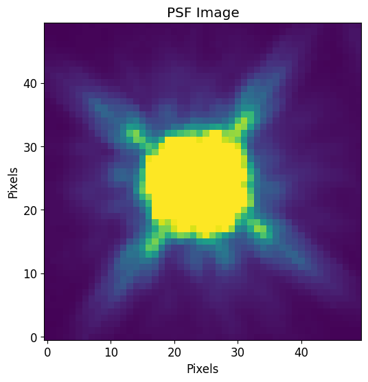
# Load PSF image (2D array)
PSF = fits.getdata('data/f105w_psf.fits.gz')

# Normalize PSF
PSF = PSF / PSF.sum()

# Note that the PSF shape is odd on all sides
print("PSF Shape = {}".format(PSF.shape))

# Plot PSF and use vmax and vmin to show difraction spikes
plt.imshow(PSF, vmin=0, vmax=PSF.std()/10)
plt.title("PSF Image")
plt.xlabel("Pixels")
plt.ylabel("Pixels")
plt.show()

PSF Shape = (50, 50)

# PSFConvolvedModel2D
psf_sersic_model = pf.PSFConvolvedModel2D(sersic_model, psf=PSF, oversample=4)

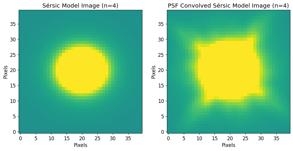
Converting Models to Images

To convert any 2D model (Astropy or PetroFit) to an image use the model_to_image function.

# Size of model image
size = 40

# sersic model image
model_image = pf.model_to_image(model=sersic_model, size=size)

# PSF convolved model image
psf_model_image = pf.model_to_image(model=psf_sersic_model, size=size)

Plot model image

fig, axs = plt.subplots(1,2, figsize=(12, 6))

plt.sca(axs[0])
plt.imshow(model_image, vmin=vmin, vmax=vmax)
plt.title('Sérsic Model Image (n=4)')
plt.xlabel("Pixels")
plt.ylabel("Pixels")

plt.sca(axs[1])
plt.imshow(psf_model_image, vmin=vmin, vmax=vmax)
plt.title('PSF Convolved Sérsic Model Image (n=4)')
plt.xlabel("Pixels")
plt.ylabel("Pixels")
plt.show()

Fitting Model to Image

We first define a PSFConvolvedModel2D model with initial guesses as follows:

sersic_model = models.Sersic2D(
        amplitude=0.1, # Intensity at r_eff
        r_eff=10, # Effective or half-lilght radius
        n=1, # Sersic index
        x_0=20, # center of model in the x direction
        y_0=20, # center of model in the y direction
        ellip=0.1, # Ellipticity
        theta=0.0, # Rotation angle in radians, counterclockwise from the positive x-axis.

        bounds=pf.get_default_sersic_bounds({'x_0': (10, 30),  'y_0': (10, 30)}), # Parameter bounds
)

psf_sersic_model = pf.PSFConvolvedModel2D(sersic_model, psf=PSF, oversample=4)

Before we fit the image, we compute the weights of each pixel using rms data as follows (please note that weights are optional and set to None by default):

fitting_weights = 1 / cutout_rms.data

Use the fit_model function to fit 2D models to images as follows:

%%time

fitted_model, fitter = pf.fit_model(
    image=cutout_image.data,
    model=psf_sersic_model,
    weights=fitting_weights,
    maxiter=10000,
    epsilon=1.4901161193847656e-08,
    acc=1e-09,
)

CPU times: user 503 ms, sys: 0 ns, total: 503 ms
Wall time: 258 ms

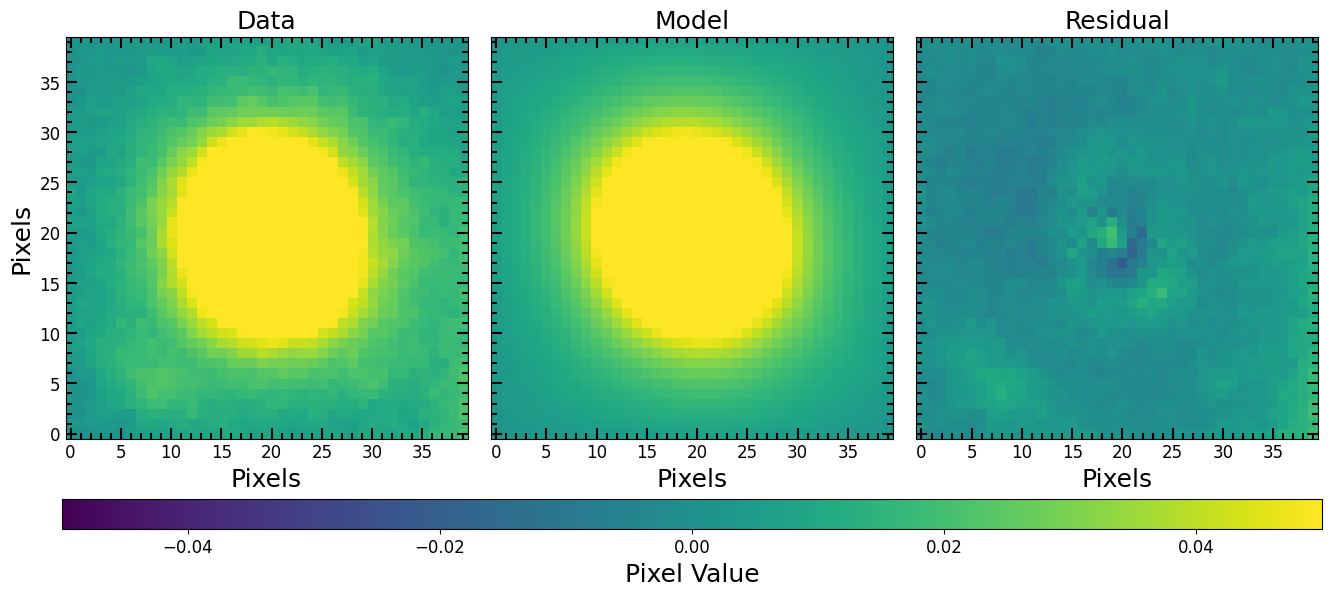
Convert the fitted model into an image

axs, cbar, model_image, residual_image = pf.plot_fit(fitted_model, cutout_image,
                                                     vmax=vmax, vmin=vmin, figsize=[6*3, 6])

plt.show()

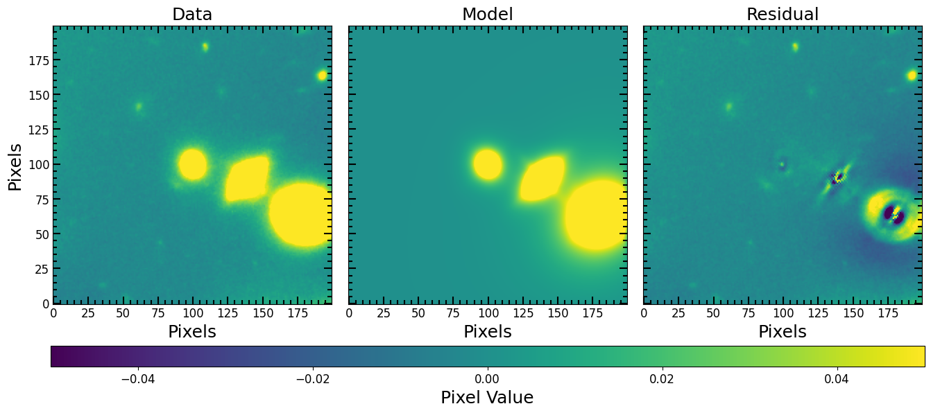
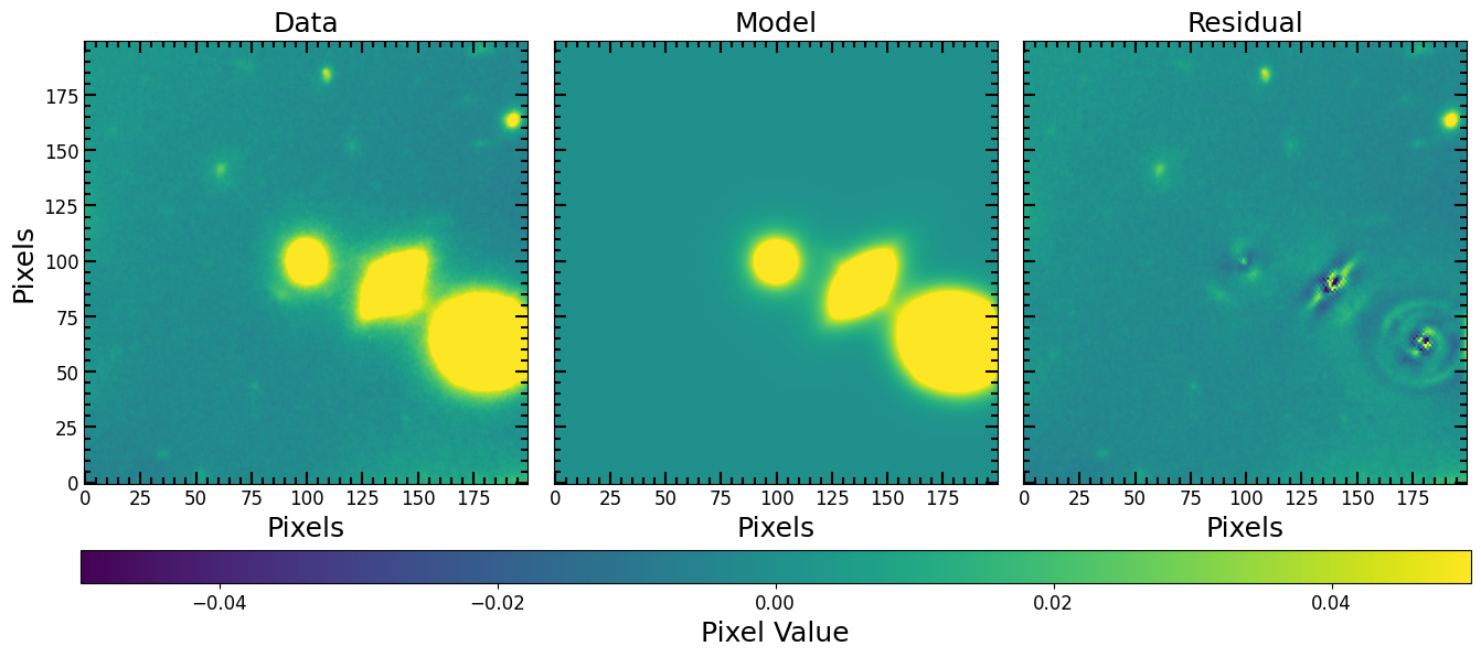
Fitting Multiple Sources

If the locations of the sources are known, we can fit all sources at the same time by creating a compound model. Note that x_0 and y_0 are known beforehand using photometric centroids. Below, a compound model of 3 Sérsic components is defined and the original image is fit (i.e. not the cutout we have been working with).

# Center elliptical galaxy we have been fitting:
galaxy_model_1 = models.Sersic2D(

        amplitude=0.1, # Intensity at r_eff
        r_eff=10, # Effective or half-lilght radius
        n=1.7384901, # Sersic index
        x_0=99.97722657736085, # center of model in the x direction
        y_0=99.12324178530918, # center of model in the y direction
        ellip=0.1, # Ellipticity
        theta=0.0, # Rotation angle in radians, counterclockwise from the positive x-axis.

        bounds=pf.get_default_sersic_bounds(), # Parameter bounds
)

# Football shaped galaxy
galaxy_model_2 = models.Sersic2D(

        amplitude=0.1, # Intensity at r_eff
        r_eff=10, # Effective or half-lilght radius
        n=1, # Sersic index
        x_0=138.56315299695075, # center of model in the x direction
        y_0=89.27757468116197, # center of model in the y direction
        ellip=0.7, # Ellipticity
        theta=0.7, # Rotation angle in radians, counterclockwise from the positive x-axis.

        bounds=pf.get_default_sersic_bounds(), # Parameter bounds
)

# Large galaxy near the bottom corner
galaxy_model_3 = models.Sersic2D(

        amplitude=0.1, # Intensity at r_eff
        r_eff=10, # Effective or half-lilght radius
        n=1, # Sersic index
        x_0=178.72302596615611, # center of model in the x direction
        y_0=63.506754312433046      , # center of model in the y direction
        ellip=0.2, # Ellipticity
        theta=0.0, # Rotation angle in radians, counterclockwise from the positive x-axis.

        bounds=pf.get_default_sersic_bounds(), # Parameter bounds
)

Make compound PSF model as follows:

compound_galaxies_model = galaxy_model_1 + galaxy_model_2 + galaxy_model_3

all_galaxies_psf_model = pf.PSFConvolvedModel2D(compound_galaxies_model, psf=PSF)

Fit the model

%%time

all_galaxies_fitted_model, fitter = pf.fit_model(
    image=image.data,
    model=all_galaxies_psf_model,
    weights=1/rms, # optional
    maxiter=10000,
    epsilon=1.4901161193847656e-08,
    acc=1e-09,
)

CPU times: user 9.19 s, sys: 74.6 ms, total: 9.27 s
Wall time: 4.99 s

pf.plot_fit(all_galaxies_fitted_model, image, vmax=vmax, vmin=vmin, figsize=[6*3, 6])
plt.show()

Looks like the bottom corner galaxy is a spiral, let us add another component for the spiral and use LevMarLSQFitter to fit again:

%%time
from astropy.modeling import fitting

# Redefine model with an extra component for galaxy 3
compound_galaxies_model = galaxy_model_1 + galaxy_model_2 + galaxy_model_3 + galaxy_model_3

# PSF model
all_galaxies_psf_model = pf.PSFConvolvedModel2D(compound_galaxies_model, psf=PSF)

# Fit the model
all_galaxies_fitted_model, fitter = pf.fit_model(
    image=image.data,
    model=all_galaxies_psf_model,
    weights=1/rms, # optional
    maxiter=100000,
    fitter=fitting.LevMarLSQFitter,
    epsilon=1.4901161193847656e-08,
    acc=1e-09,
)

# Plot the fit
pf.plot_fit(all_galaxies_fitted_model, image, vmax=vmax, vmin=vmin, figsize=[6*3, 6])
plt.show()

CPU times: user 10.5 s, sys: 11 ms, total: 10.5 s
Wall time: 10.5 s

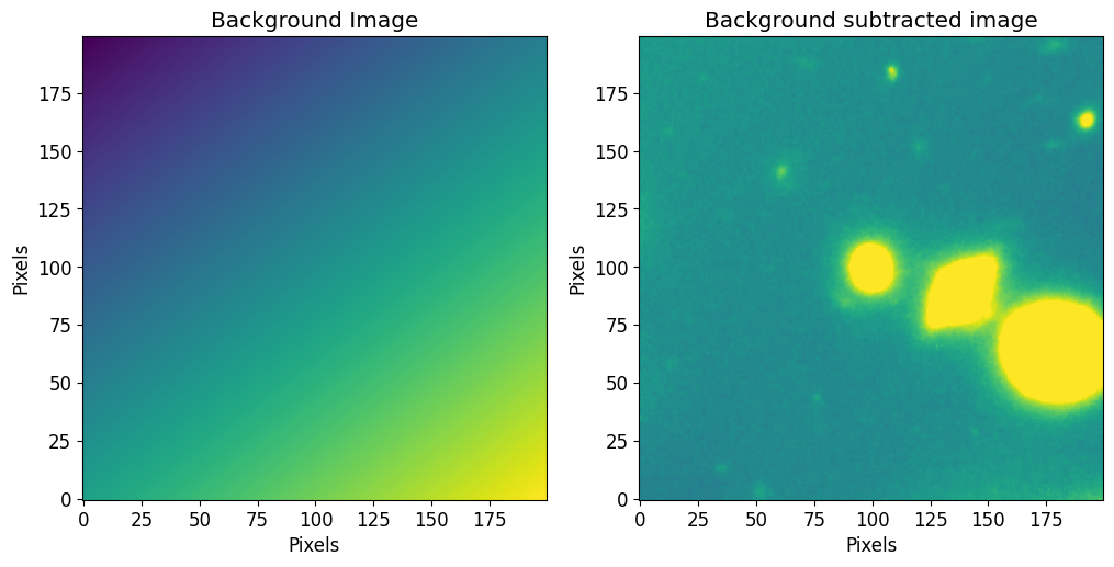
Fitting Image Backgrounds

The fit_background function can be used to fit the background pixels using a 2D plane. It will sigma clip the pixels (sigma value provided by the user) and fit a 2D plane to the clipped image. Users can also provide their own 2D models.

bg_model, fitter = pf.fit_background(image, sigma=3.0)
bg_image = pf.model_to_image(bg_model, size=(image.shape[1], image.shape[0]))

Plot backround

fig, axs = plt.subplots(1,2, figsize=[6*2, 6])

plt.sca(axs[0])
plt.imshow(bg_image)
plt.title("Background Image")
plt.xlabel("Pixels")
plt.ylabel("Pixels")

plt.sca(axs[1])
plt.imshow(image.data - bg_image, vmin=vmin, vmax=vmax)
plt.title("Background subtracted image")
plt.xlabel("Pixels")
plt.ylabel("Pixels")
plt.show()

Fitting a PSF With a Moffat Model

In this example we fit the PSF itself, from the section above, using an astropy 2D Moffat model (PSF convolution is not needed for such fits). We then use the model PSF to fit the cutout image from the Making Cutouts section. We start by initializing a Moffat2D model:

moffat_model = models.Moffat2D(amplitude=1, x_0=25, y_0=25, gamma=1, alpha=1)

Fit the model using fit_model:

%%time

fitted_moffat_model, fitter = pf.fit_model(
    image=PSF,
    model=moffat_model,
    weights=None, # optional
    maxiter=10000,
    epsilon=1.4901161193847656e-08,
    acc=1e-09,
)

CPU times: user 4.9 ms, sys: 983 μs, total: 5.88 ms
Wall time: 5.75 ms

Plot the fit and print out fitted parameters:

psf_vmax = PSF.std()/10
psf_vmin = -psf_vmax
pf.plot_fit(fitted_moffat_model, PSF, vmin=psf_vmin, vmax=psf_vmax, figsize=[6*3, 6])
plt.show()

print("Fitted Moffat Params:")
pf.print_model_params(fitted_moffat_model)

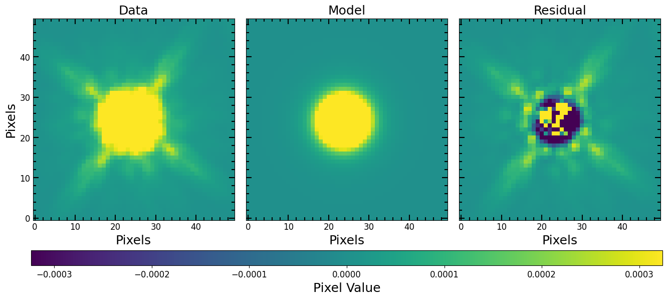
Fitted Moffat Params:
0.0780  amplitude
23.6932 x_0
24.0988 y_0
2.2447  gamma
2.3227  alpha

Use the fitted Moffat model as a PSF and fit a galaxy:

# Make Moffat PSF
moffat_model_psf = pf.model_to_image(fitted_moffat_model, size=(51, 51))

# Make a PSFConvolvedModel2D model with Moffat PSF
moffat_psf_sersic_model = pf.PSFConvolvedModel2D(
    sersic_model,
    psf=moffat_model_psf, # Moffat PSF
    oversample=4
)

# Fit the galaxy cutout image
fitted_moffat_psf_sersic_model, fitter = pf.fit_model(
    image=cutout_image.data,
    model=moffat_psf_sersic_model,
    weights=fitting_weights, # optional
    maxiter=10000,
    epsilon=1.4901161193847656e-08,
    acc=1e-09,
)

pf.plot_fit(fitted_moffat_psf_sersic_model, cutout_image.data, vmin=vmin, vmax=vmax, figsize=[6*3, 6])
plt.show()

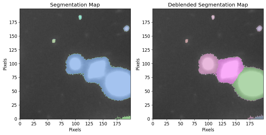
Making a Photutils Source Catalog

To make a Photutils source catalog, which can also be converted into a table, use the make_catalog wrapper as follows:

from astropy.stats import sigma_clipped_stats

# Sigma clipped stats
image_mean, image_median, image_stddev = sigma_clipped_stats(image.data, sigma=3)

cat, segm, segm_deblend = pf.make_catalog(
    image=image.data,  # Input image
    threshold=image_stddev*3,  # Detection threshold
    deblend=True,  # Deblend sources?
    npixels=4**2,  # Minimum number of pixels that make up a source
    plot=True, vmax=vmax, vmin=vmin, # Plotting params
    figsize=(12, 6)
)

Display sources catalog as table:

cat.to_table()

QTable length=8

label	xcentroid	ycentroid	sky_centroid	bbox_xmin	bbox_xmax	bbox_ymin	bbox_ymax	area	semimajor_sigma	semiminor_sigma	orientation	eccentricity	min_value	max_value	local_background	segment_flux	segment_fluxerr	kron_flux	kron_fluxerr
								pix2	pix	pix	deg
int32	float64	float64	object	int64	int64	int64	int64	float64	float64	float64	float64	float64	float64	float64	float64	float64	float64	float64	float64
1	61.08347174238899	141.05186559012205	None	59	64	138	144	34.0	1.7994370638925237	1.2826901873829257	72.98283673407356	0.7013382917172669	0.010554540902376175	0.026845833286643028	0.0	0.5834723142907023	nan	1.8317878434947907	nan
2	192.36299560404697	163.40391871827393	None	187	197	158	169	86.0	2.3144983589944554	1.9834471217713212	53.655204869988644	0.5153724293039628	0.010591089725494385	0.0929785966873169	0.0	2.8758262349292636	nan	3.270753741333536	nan
3	108.72693550508657	183.8851479597333	None	106	111	180	187	37.0	1.8003927404449662	1.257057560548163	-87.14736406479223	0.7158901102937193	0.010464809834957123	0.045437149703502655	0.0	0.8372195269912481	nan	1.0690440471675258	nan
4	176.59884904430535	1.7105077906435575	None	172	181	0	5	22.0	2.5652493504083584	1.2345618770639404	13.128240218386493	0.876575763829376	0.010684505105018616	0.01434874627739191	0.0	0.26085690688341856	nan	3.44449120866383	nan
5	192.09296727764394	1.82553577948899	None	180	199	0	7	84.0	4.976606287872485	1.5422939287464803	5.980651162675711	0.9507662987626069	0.010602000169456005	0.02371048368513584	0.0	1.247399945743382	nan	3.590573711610179	nan
6	178.73633119059068	63.493826518219336	None	143	199	33	95	2704.0	9.40299866437019	9.177157386885888	-48.66212288913661	0.21785120428951427	0.010437765158712864	3.6771397590637207	0.0	421.7741427142173	nan	422.6815556552462	nan
7	138.55898473281684	89.25004484979968	None	109	166	63	112	1864.0	7.532153967377171	5.563519557842017	44.31309259442659	0.6741045627289916	0.010432953014969826	3.6545557975769043	0.0	244.33296140562743	nan	240.57513423073874	nan
8	99.92859014542458	99.15188824983441	None	83	118	80	118	1114.0	6.7507255757709	6.379388610260266	76.6082699457646	0.32709046915385503	0.010427203960716724	0.44580602645874023	0.0	56.775723142549396	nan	60.32600669722427	nan

Curve of Growth and Petrosian Radii

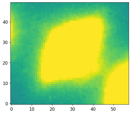
This step in detailed in the Photometry and Petrosian sections but we will do a simple example here. The first step is to pick a source from the catalog we made in the last step:

source = cat[6]

# Photutils cutout of the source
# Not to be confused with the cutout we made
plt.imshow(source.data, vmin=vmin, vmax=vmax)
plt.show()

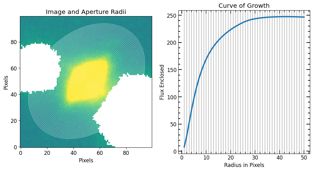
Now we use PetroFit source_photometry to compute the curve of growth

r_list = pf.make_radius_list(
    max_pix=50, # Max pixel to go up to
    n=50 # the number of radii to produce
)

# Photomerty
flux_arr, area_arr, error_arr = pf.source_photometry(

    # Inputs
    source, # Source (`photutils.segmentation.catalog.SourceCatalog`)
    image.data, # Image as 2D array
    segm_deblend, # Deblended segmentation map of image
    r_list, # list of aperture radii

    # Options
    cutout_size=max(r_list)*2, # Cutout out size, set to double the max radius
    bg_sub=True, # Subtract background
    sigma=3, sigma_type='clip', # Fit a 2D plane to pixels within 3 sigma of the mean
    plot=True, vmax=vmax, vmin=vmin, # Show plot with max and min defined above
)
plt.show()

7

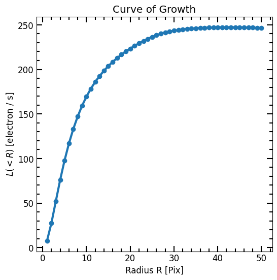
Now we have a radius list (r_list) and a corresponding enclosed flux list (flux_arr), we can plot the curve of growth and initialize a Petrosian profile

plt.plot(r_list, flux_arr, linewidth=3, marker='o')

pf.mpl_tick_frame()

plt.title("Curve of Growth")
plt.xlabel("Radius R [Pix]")
plt.ylabel("$L(<R)$ [{}]".format(image.unit))
plt.show()

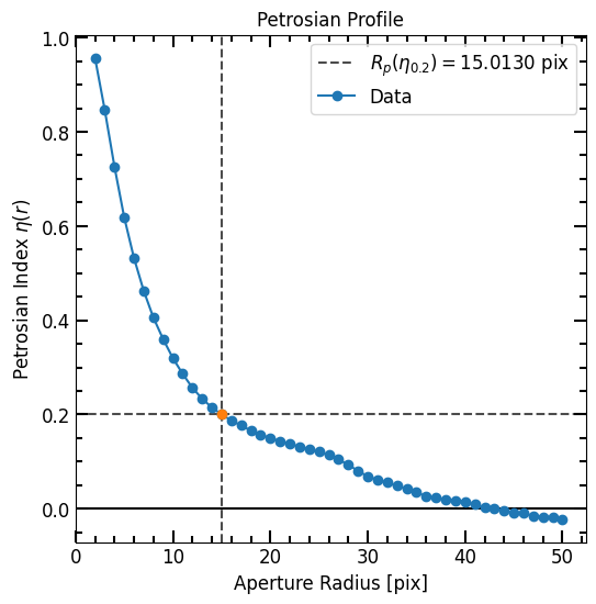
We now define the Petrosian using the curve of growth arrays and inspect various radii:

p = pf.Petrosian(r_list, area_arr, flux_arr)

print(p.r_half_light, p.r_total_flux, p.r_petrosian, p.c2080)

6.361672334466893 30.02360472094419 15.013002600520105 3.376753454810066

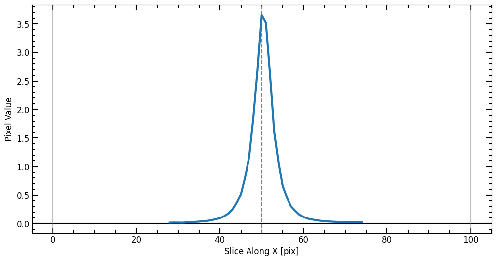
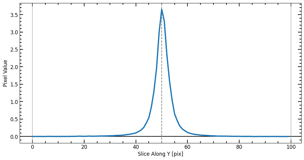
The radii can be plotted as follows:

# Plot Petrosian
p.plot(plot_r=True)
plt.show()