Correction Grids

Correction grids can be thought of as lookup tables that provide corrected Petrosian derived values. These grids are typically generated through simulations or theoretical models to offer the best correction for Petrosian profiles. This section discusses the concept of correction grids: how they’re generated, when and why they should be used, and how they enhance accuracy.

Necessity and Implications

Are Correction Grids Always Needed?

The short answer is no, but they are very useful in some cases. Petrosian corrections offer more precise measurements of galaxies. The necessity hinges on your data quality, research goals, and desired precision. Here are key considerations on why the default settings are usually good enough:

1. Standard Practices: Numerous studies, such as those from the Sloan Digital Sky Survey (SDSS), rely on default settings. The parameters \(\eta = 0.2\) and \(\epsilon = 2\) are widely accepted because they typically produce reliable results across many scenarios.

2. Noise Constraints: If the fainter parts of galaxies in your images are submerged below the noise level, detailed corrections might not significantly impact the outcome since that portion of the galaxy is not meaningfully measurable. Here, the additional steps and computational demands of correction grids might be unwarranted.

3. Practical Implications: While correction grids can produce improved results, they require optimal background subtraction. Not all datasets might meet this standard.

Correction grids promise enhanced precision but aren’t always essential. For a majority of cases, default settings suffice.

When are Correction Grids Needed?

While the default settings serve most general purposes, there are specific scenarios where correction grids are beneficial:

1. Galaxy Size Estimation: If your research aims to measure the size of a galaxy which suffers due to poor signal-to-noise, you can estimate its total flux radius based on the corrected epsilon. Remember, this isn’t about recovering the total flux which includes regions submerged under noise, but about the estimating the full extent of the galaxy based on the measurable components of the light profile.

2. Estimating Sérsic Index: Correction grids can be used to estimate the Sérsic index of single component galaxies.

3. High-Precision Studies: For projects that require a granular study of galaxy structures, or when analyzing galaxies with distinct features that might get overlooked with standard parameters, correction grids provide the extra precision that may be needed.

4. Superior Data Quality: If you have high-quality images with excellent background subtraction and reasonable signal-to-noise ratios, the total flux can be estimated to higher accuracy. That is, high quality data allows you to measure the flux up to the corrected total flux radius.

In essence, when the goal shifts from general measurements to intricate, high-resolution studies of galactic structures and sizes, correction grids become a useful tool.

Generating a Correction Grid

Correction grids are essentially lookup tables that map certain observational properties of a galaxy (like Petrosian radius, uncorrected half light radius, and concentration indices) to more intrinsic properties (like Sérsic index and the corrected epsilon value). In this section, we’ll walk through the steps of creating a correction grid.

To start with PetroFit, simply import it as follows:

import petrofit as pf

Load PSF (Optional)

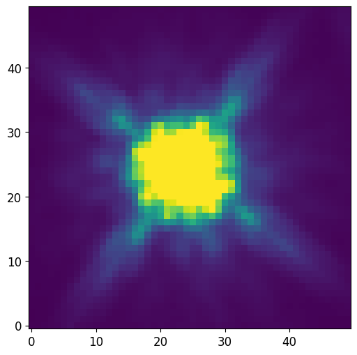
We load an HST F105W PSF and normalize it to sum to 1:

from matplotlib import pyplot as plt

plt.rcParams['figure.figsize'] = [6, 6]
plt.rcParams['image.origin'] = 'lower'
plt.rcParams['font.size'] = 12

from astropy.io import fits

# Load PSF image (2D array)
PSF = fits.getdata('data/f105w_psf.fits.gz')

# Normalize PSF
PSF = PSF / PSF.sum()

# Note that the PSF shape is odd on all sides
print("PSF Shape = {}".format(PSF.shape))

# Plot PSF and use vmax and vmin to show difraction spikes
plt.imshow(PSF, vmin=0, vmax=5e-4)
plt.show()

PSF Shape = (50, 50)

Define Sampling Points

The correction grid is generated along with a set of half-light radii and Sersic indices. The generator loops through the Sersic indices for each half-light radius in the radius list. For this documentation, we define a small set of values, with the Sersic indices of a Gaussian and de Vaucouleurs’ profile.

import numpy as np

r_eff_list = np.array([7, 10, 15])
n_list = np.array([0.5, 1., 4.])

Grid Simulation

We do a simple API call to generate the correction grid. We provide a PSF and oversampling rule as well. Oversampling becomes important for small half-light radii since the model needs to be sampled well in the center.

The generate_petrosian_sersic_correction grid follows the following steps to generate the correction grid:

• Computes the total flux (total_flux) of an ideal Sersic profile with the sampling points using the petrofit.modeling.models.sersic_enclosed function and setting the radius to np.inf.

• Computes the radius equal to total_flux * 0.99.

• Makes a PSF convolved Sersic Model image and measures the photometry.

• Measures the uncorrected Petrosian radius.

• Computes the correct epsilon value as corrected_epsilon = r(total_flux) / r_petrosian.

• It also saves other values, such as the uncorrected C2080 which can be used to map to the Sersic index.

output_file_name='temp/example_correction_gid.ecsv'

petrosian_grid = pf.generate_petrosian_sersic_correction(
    output_file_name=output_file_name, # Output file name
    psf=PSF, # PSF (optional)
    r_eff_list=r_eff_list, # List of r_e to sample
    n_list=n_list, # List of n to sample
    oversample=4, # Oversample factor or region, see fitting docs
    out_format='ascii.ecsv', # Output format, should match file name
    overwrite=True, # Overwrite output
    ipython_widget=True, # Progress bar
    n_cpu=None, # int value for number of mp threads
    plot=False, # Plot each step, can not be True if n_cpu > 1

)

petrosian_grid

Table length=9

n	r_eff	sersic_r_20	sersic_r_80	sersic_r_99	sersic_L_inf	p02	p03	p04	p05	p0502	p0302	u_epsilon	u_epsilon_50	u_epsilon_80	u_r_50	u_r_99	u_r_20	u_r_80	u_c2080	u_c5090	c_epsilon	c_epsilon_50	c_epsilon_80	c_r_50	c_r_99	c_r_20	c_r_80	c_c2080	c_c5090
float64	int64	float64	float64	float64	float64	float64	float64	float64	float64	float64	float64	float64	float64	float64	float64	float64	float64	float64	float64	float64	float64	float64	float64	float64	float64	float64	float64	float64	float64
0.5	7	3.9494261674515654	10.535743151744386	18.04297517869382	22208.564694953242	16.690338067613524	14.742948589717944	13.191638327665533	11.816363272654531	0.7499064971159685	0.2694039121096147	2.0	0.4702462995145921	0.7427218793072451	7.848569713942788	33.38487697539508	4.402680536107221	12.39627925585117	2.247870887683088	1.477215403931874	1.5838256474738557	0.4676574579013603	0.7294770646895044	7.805361072214443	26.43908781756351	4.3810762152430485	12.255851170234047	2.2338133500139796	1.443311364049927
0.5	10	5.6420373820736645	15.051061645349122	25.77567882670543	45323.60141827192	22.48849769953991	19.885377075415082	17.75975195039008	15.834366873374675	0.761798705625901	0.267133067590084	2.0	0.4798345490126312	0.7461928482476425	10.790758151630326	44.98239647929586	6.0778155631126225	16.780756151230243	2.2053200481575006	1.398916647555213	1.3667428966087338	0.47645436755025794	0.729443744213396	10.714742948589718	30.737147429485894	6.047409481896379	16.567913582716542	2.1884922205394455	1.3671755462140593
0.5	15	8.463056073110499	22.576592468023684	38.66351824005819	101978.10319111182	32.02240448089618	28.364672934586917	25.30506101220244	22.521504300860173	0.7642827173570272	0.26338079339405823	2.0	0.4898488255872064	0.7547663668165917	15.686137227445489	64.05461092218442	8.86757351470294	24.169433886777355	2.1773084029854246	1.3534094001636479	1.2911297807635969	0.4862881059470265	0.736866400939908	15.572114422884576	41.341268253650725	8.821964392878575	23.8501700340068	2.159630895166948	1.3247894047084208
1.0	7	3.4152455989729886	12.269877985786641	27.687042520030552	10929.805669580057	18.977595519103822	15.490898179635927	12.917383476695338	10.841968393678735	1.2156652456010393	0.4408229332439093	2.0	0.42609282273450755	0.7614605403240257	8.08621724344869	37.95659131826365	4.067413482696539	14.450690138027605	2.752851323921932	1.854400745123529	1.6516698747257175	0.4226354235841001	0.7417938655072812	8.020604120824164	31.346069213842767	4.051010202040407	14.25385077015403	2.7318443537737207	1.8246976026729558
1.0	10	4.8789222842471265	17.52839712255235	39.552917885758006	22305.725856285833	25.280656131226245	20.63872774554911	17.068013602720544	14.11622324464893	1.265349116905938	0.44052709634619963	2.0	0.43544762537783477	0.7715820791593473	11.008401680336068	50.56991398279656	5.508501700340068	19.506101220244048	2.745684928420304	1.8121310726092839	1.641241793161436	0.43264650492965545	0.7487453452425344	10.9375875175035	41.482096419283856	5.484896979395879	19.24644928985797	2.7259107247705625	1.7791529983794634
1.0	15	7.31838342637069	26.292595683828527	59.32937682863701	50187.88317664311	35.513302660532105	28.92758551710342	23.79355871174235	19.473894778955792	1.3046912176308711	0.44539438244001306	2.0	0.4465191994637556	0.7895353487559919	15.857371474294858	71.0268053610722	7.900580116023204	28.03900780156031	2.75051830028121	1.8075396077736015	1.700997857031393	0.4435450710016842	0.7676036327672117	15.751750350070013	60.39427885577115	7.865373074614922	27.722144428885773	2.7355374733767586	1.7796966409157084
4.0	7	1.9338894613170134	21.37899838138344	132.60580887212956	51.861320264524814	20.729545909181834	12.735347069413882	8.928585717143427	6.782956591318263	2.4258537551641766	1.0578950185789684	2.0	0.368581547280149	0.8897584606328467	7.640528105621124	41.4624924984997	2.926785357071414	18.444288857771554	3.997355207847013	2.6804143543491543	7.164423510366633	0.42169511806768517	1.1173986772316422	8.741548309661933	148.50230046009202	3.167633526705341	23.91498299659932	4.3896757273607	3.312617849643298
4.0	10	2.7626992304528764	30.541426259119202	189.43686981732796	105.83942911127511	25.805161032206442	15.783156631326266	10.442088417683536	7.621524304860972	2.6483236731181488	1.0675635354491433	2.0	0.3794728682170542	0.9125736434108527	9.792358471694339	51.60092018403681	3.631726345269054	23.549109821964393	4.05930689273775	2.6732303489915554	7.8467121681302565	0.4490077519379845	1.2233150416937433	11.586717343468694	202.50650130026006	3.990598119623925	32.7003400680136	4.567571377813081	3.4406515906900377
4.0	15	4.144048845679315	45.8121393886788	284.15530472598925	238.138715500369	33.366673334666935	20.404080816163233	12.882576515303061	8.881776355271054	2.8740653809355003	1.0679793726990117	2.0	0.39595923261390886	0.9509232613908873	13.211842368473695	66.76835367073416	4.671534306861373	31.729145829165837	4.159994190872208	2.664062476224748	8.860372029430788	0.48925059952038374	1.3916191368348632	16.3246649329866	295.6805361072215	5.310062012402481	48.17123424684937	4.788440905285227	3.559459521262453

PetrosianCorrection

The PetrosianCorrection class is designed to compute corrections for Petrosian based on default Petrosian measurements.

Loading and Navigating

1. Grid Input: To initialize the PetrosianCorrection class, you’ll need a correction grid. This grid is typically an Astropy Table that has been generated with the function petrofit.correction.generate_petrosian_sersic_correction.

# Input generated grid table
pc = pf.PetrosianCorrection(petrosian_grid)

2. Reading and Writing Grids:

   • Use the PetrosianCorrection.read(file_path) class method to read a correction grid from a file.

   • Similarly, to save your correction grid to a file, utilize the write(grid_file, file_format=None) method.

# Read F105W grid:
pc = pf.PetrosianCorrection.read(output_file_name)

3. Working with Grid Data:

   • The grid_keys property will provide you with the column names of your grid.

   • Use unique_grid_values(key) to obtain unique values from a specific column.

   • The filter_grid(key, value) method helps filter the grid based on a specific key and value.

# Read ideal Sersic grid:
pc = pf.PetrosianCorrection.read('data/no_psf_corr.ecsv')

print(pc.grid_keys)

['n', 'r_eff', 'sersic_r_20', 'sersic_r_80', 'sersic_r_99', 'sersic_L_inf', 'p02', 'p03', 'p04', 'p05', 'p0502', 'p0302', 'u_epsilon', 'u_epsilon_50', 'u_epsilon_80', 'u_r_50', 'u_r_99', 'u_r_20', 'u_r_80', 'u_c2080', 'u_c5090', 'c_epsilon', 'c_epsilon_50', 'c_epsilon_80', 'c_r_50', 'c_r_99', 'c_r_20', 'c_r_80', 'c_c2080', 'c_c5090']

# List all Sersic indices available
pc.unique_grid_values('n')

array([0.5, 0.6, 0.7, 0.8, 0.9, 1. , 1.1, 1.2, 1.3, 1.4, 1.5, 1.6, 1.7,
       1.8, 1.9, 2. , 2.1, 2.2, 2.3, 2.4, 2.5, 2.6, 2.7, 2.8, 2.9, 3. ,
       3.1, 3.2, 3.3, 3.4, 3.5, 3.6, 3.7, 3.8, 3.9, 4. ])

# Provide rows for a grid key's value
# For example all rows with n=1
pc.filter_grid('n', 1.)

Table length=9

n	r_eff	sersic_r_20	sersic_r_80	sersic_r_99	sersic_L_inf	p02	p03	p04	p05	p0502	p0302	u_epsilon	u_epsilon_50	u_epsilon_80	u_r_50	u_r_99	u_r_20	u_r_80	u_c2080	u_c5090	c_epsilon	c_epsilon_50	c_epsilon_80	c_r_50	c_r_99	c_r_20	c_r_80	c_c2080	c_c5090
float64	int64	float64	float64	float64	float64	float64	float64	float64	float64	float64	float64	float64	float64	float64	float64	float64	float64	float64	float64	float64	float64	float64	float64	float64	float64	float64	float64	float64	float64
1.0	8	3.903137827397701	14.02271769804188	31.642334308606404	14275.66454802293	19.079815963192637	15.621124224844968	12.960592118423683	10.7751550310062	1.24075326958047	0.43430947634475076	2.0	0.4229712728035228	0.7580520025162508	8.070214042808562	38.156231246249256	3.9709941988397683	14.463492698539708	2.806869640376674	1.8544905387612654	1.6635968566174741	0.4200146781295869	0.7394995983492405	8.01380276055211	31.744148829765955	3.9521904380876176	14.294258851770355	2.7916188964442834	1.8240139508932398
1.0	10	4.8789222842471265	17.52839712255235	39.552917885758006	22305.725856285833	23.4000800160032	19.02000400080016	15.6873374674935	12.902180436087217	1.2927711564687436	0.45003369259072135	2.0	0.4311018405327543	0.7720577549432794	10.087817563512703	46.79315863172634	4.941988397679536	18.06621324264853	2.8148270530153314	1.8511364392182104	1.6934398809058022	0.4280756046060336	0.7516043950341623	10.017003400680135	39.61732346469294	4.918383676735347	17.85377075415083	2.7995377478760726	1.8226683398980135
1.0	12	5.854706741096551	21.03407654706282	47.463501462909605	32120.24523305159	27.69033806761352	22.426885377075415	18.393478695739148	15.046609321864372	1.324448065773273	0.45779647311977595	2.0	0.43618881118881125	0.7818947581344277	12.078215643128626	55.36847369473895	5.942588517703541	21.650930186037208	2.8075045007676285	1.8531091616278847	1.7161049249721019	0.4341371438478877	0.7602037138858923	12.021404280856173	47.52850570114023	5.9141828365673135	21.42368473694739	2.7949971110740517	1.821616418480862
1.0	14	6.830491197945977	24.539755971573282	55.374085040061104	43719.22267832023	32.00360072014403	25.85677135427085	21.113022604520904	17.204440888177633	1.3477914001867675	0.4631227419782593	2.0	0.44005725500981335	0.7897253509682097	14.083416683336667	63.99299859971995	6.910782156431286	25.27405481096219	2.815738598797761	1.851949792465929	1.7315751890597235	0.4379820734314252	0.7679413801628006	14.017003400680135	55.42568513702741	6.877575515103021	24.9751950390078	2.8003676042616044	1.8225760596660439
1.0	16	7.806275654795402	28.04543539608376	63.28466861721281	57102.65819209172	36.333066613322664	29.263052610522106	23.85657131426285	19.319663932786558	1.3715124376691632	0.46991213492826367	2.0	0.44258901386893057	0.7945151930583774	16.080616123224644	72.67993598719744	7.882176435287058	28.86717343468694	2.818790547772201	1.8526426866865697	1.7426662208475252	0.44051885987369865	0.7730898321507773	16.005401080216046	63.31566313262653	7.882176435287058	28.566313262652532	2.796040212517563	1.8257252368835972
1.0	18	8.782060111644828	31.55111482059424	71.19525219436454	72270.5517743661	40.62812562512502	32.70654130826165	26.58531706341268	21.484296859371874	1.3835282102063495	0.4709608320425094	2.0	0.44565731166912853	0.7989807976366322	18.10622124424885	81.26765353070614	8.89517903580716	32.46109221844369	2.811042173832883	1.8502334979631763	1.7529220087684552	0.442712949286066	0.7773946798423912	17.986597319463893	71.21924384876975	8.835367073414684	32.102220444088815	2.801552376569915	1.8275981446613496
1.0	20	9.757844568494253	35.0567942451047	79.10583577151601	89222.90342514333	44.94898979795959	36.06721344268854	29.285857171434287	23.584716943388678	1.400446336620199	0.47803672848363443	2.0	0.4480596350689809	0.8020160213618158	20.13982796559312	89.88057611522305	9.852170434086817	36.0498099619924	2.8168553175362727	1.8455182550741536	1.7602328886954623	0.4453983088562528	0.780159123080737	20.020204040808164	79.11442288457691	9.852170434086817	35.69093818763753	2.79513024003569	1.8223189749430866
1.0	22	10.73362902534368	38.56247366961518	87.01641934866778	107959.71314442341	49.26985397079416	39.4878975795159	31.98639727945589	25.74514902980596	1.4094293246735825	0.4805863175274263	2.0	0.44882663418595214	0.8045188794153472	22.11362272454491	98.55331066213243	10.868973794758952	39.63852770554111	2.809644867201815	1.8500325232830082	1.7662796953140032	0.446398700771417	0.7831493521543753	21.993998799759954	87.00960192038409	10.809161832366474	39.27965593118624	2.801878279462548	1.8264491340662061
1.0	24	11.709413482193103	42.06815309412564	94.92700292581921	128480.98093220637	53.59071814362873	42.90858171634327	34.68693738747749	27.905581116223246	1.4169925299929624	0.48272708543732895	2.0	0.4505860395670026	0.8066181410974245	24.147229445889177	107.16623324664933	11.825965193038607	43.22724544908982	2.814604828183506	1.8461171094724786	1.7715130861326402	0.4483538633818589	0.7855263022709479	24.02760552110422	94.96459291858372	11.766153230646129	42.80856171234247	2.804480683450517	1.8221464723407068

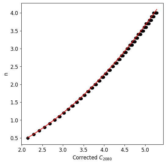
# Plotting relations
pc_c_c2080_list = np.sort(pc.unique_grid_values('c_c2080')) # Get corrected c_c2080
approx_n_values = pf.PetroApprox.c2080_to_n(pc_c_c2080_list) # Get n from PetroApprox for comparison

# Plot
plt.scatter( pc.grid['c_c2080'], pc.grid['n'], color='black')
plt.plot(pc_c_c2080_list, approx_n_values, color='red')

plt.xlabel('Corrected $C_{2080}$')
plt.ylabel('n')
plt.show()

Correcting a Petrosian Profile

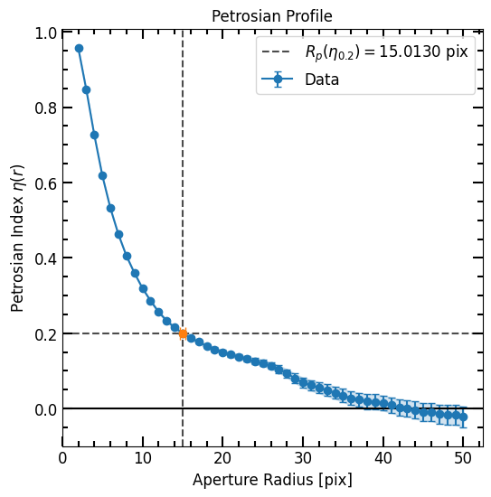
In the Photometry Chapter we constructed a curve of growth for the football shaped galaxy:

import numpy as np
from astropy.table import Table
phot_table = Table.read('data/abell_2744_galaxy_f105w_photometry.ecsv') # Read table

# Load data
r_list = np.array(phot_table['r_list'])
flux_arr = np.array(phot_table['flux_arr'])
area_arr = np.array(phot_table['area_arr'])
error_arr = np.array(phot_table['error_arr'])


# Make Petrosian profile
p = pf.Petrosian(r_list, area_arr, flux_arr, flux_err=error_arr)

p.plot()
plt.show()

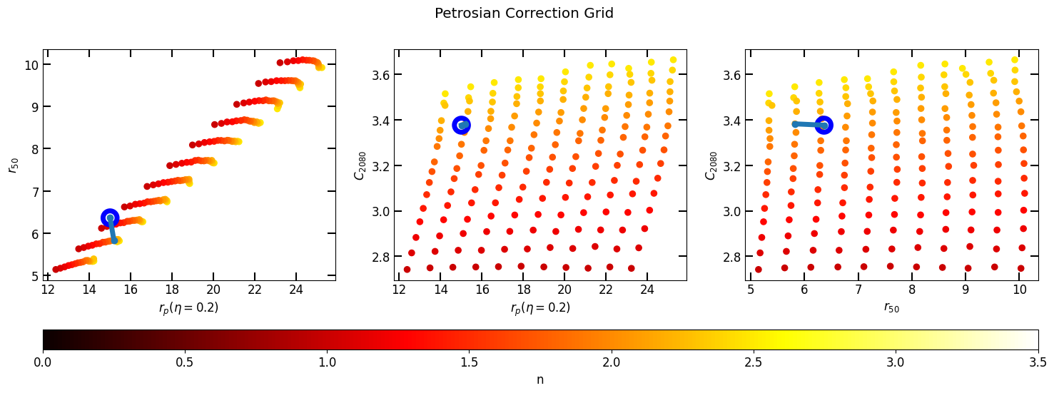
1. Correct Profile:

   • Simply use the correct(p) function to correct the profile.

   • Use plot_correction function to see the closest value.

   • The parameters used for correction are derived directly from the grid. Specifically:

     • 'p02': Represents the Petrosian radius \(P_{02} = R(\eta_{0.2})\).

     • 'u_r_50': Stands for the uncorrected half-light radius.

     • 'u_c2080': Corresponds to the uncorrected concentration index.

pc = pf.PetrosianCorrection.read('data/f105w_psf_corr.ecsv')

# Plot grid and uncorrected profile on grid (p)
pc.plot_correction(p)
plt.show()

# Pass uncorrected p to the correct function
p_corrected = pc.correct(p)

# Plot corrected profile
p_corrected.plot()
plt.show()

2. Estimating Parameters:

   • The method estimate_n(p) will give an estimated Sérsic index n based on the half-light radius and c2080 computed using the default epsilon value.

   • The method estimate_epsilon(p) will provide a corrected epsilon value given the half-light radius and c2080 computed with the default epsilon.

n = pc.estimate_n(p)
n

np.float64(2.1)

corr_epsilon = pc.estimate_epsilon(p)
corr_epsilon

np.float64(2.227805629021434)