Background Information
Introduction
Measuring true sizes and fluxes of galaxies has always posed challenges due to varying morphology, proximity to neighboring galaxies, and low surface brightness features. Several methods have been proposed to estimate galaxy fluxes, shapes, and angular sizes. Key among these is the analysis of the light distribution profile of a galaxy.
Parametric Descriptions:
De Vaucouleurs (1948) first introduced a power-law profile, employing an exp\([{-kr^{1/4}}]\) intensity profile for elliptical galaxies.
Sérsic (1963, 1968) later generalized this to describe galaxies of various morphologies.
Petrosian Profile:
Proposed by Petrosian (1976), it offers a distance-independent method for measuring galaxy radii. It’s useful in determining radial concentrations of galaxy light profiles and in estimating parameters of Sérsic profiles.
PetroFit Package:
PetroFit, leveraging Astropy and Photutils, is aimed at computing Petrosian radii and magnitudes.
It prioritizes accurate measurements within the Astropy ecosystem and incorporates correction grids as described by Crawford (2006).
Beyond Petrosian profiles, it offers robust parameter fitting based on Astropy models.
In the sections ahead, we will detail the morphological properties measurable with PetroFit.
Sérsic Profiles
The Sérsic profile is a mathematical function that describes how the intensity of a galaxy varies with radius r from its center. The profile can be described using the following formulation:
\(I\left( r(x,y) \right) = I_e\exp\left\{-b_n\left[\left(\frac{r}{r_{e}}\right)^{(1/n)}-1\right]\right\}\)
The total flux within a radius r is given by the following integral:
\(L(\leq r) = 2 \pi \int_{0}^{r} I(r^\prime) r^\prime dr^\prime\)
Where:
\(I\) is the intensity or flux at position
(x, y).\(r\) is the radius (angular) from the center that corresponds to
(x, y).\(r_{e}\) is the effective radius which is equal to the half-light radius.
\(I_e\) is the flux at the half light radius or \(I_e = I(r_{e})\).
\(n\) is the Sérsic index which determines the “steepness” of the profile.
n = 4corresponds to a de Vaucouleurs’ profile whilen = 1gives the exponential profile.
The constant \(b_n\) is defined such that \(r_e\) contains half the total flux, and can be solved for numerically using:
\(\Gamma(2n) = 2\gamma (2n,b_n)\)
In python, the Sérsic \(b_n\) can be calculated as follows:
[1]:
from scipy.special import gammaincinv
n = 4 # Sersic index
b_n = gammaincinv(2. * n, 0.5)
Ellipticity and Elongation
Galaxies that can be described with a Sérsic profile are usually not perfectly symmetrical and often display an elliptical distribution. We define two quantities that can be used to describe the elliptical components of galaxies. Ellipticity and elongation are defined as follows:
\(ellip = 1 - \frac{b}{a} = \frac{elong - 1}{elong}\)
\(elong = \frac{a}{b} = \frac{1}{1 - ellip}\)
Where \(a\) is the unit length of the semi-major axis and \(b\) is the corresponding semi-minor axis. A circle corresponds to \(ellip = 0\) and \(elong = 1\). Ellipticity ranges from 0 to 1 while elongation ranges from 1 to infinity. The SExtractor and Photutils packages use elongations for apertures while the Astropy-modeling sub-module uses ellipticity for Sérsic models.
Input Radius
Elliptical Sérsic profiles can be described using \(ellip\) (ellipticity) and \(\theta\) (rotation angle). In such cases, the radius is given by the following expression:
\(r(x, y, \theta, ellip) = \sqrt{\left(r_{maj}(x, y)\right)^2 - \left(\frac{r_{min}(x, y)}{(1 - ellip)}\right)^2}\)
Where:
\(r_{maj}(x, y) = (x - x_0)\cdot{cos(\theta)} + {(y - y_0)}\cdot sin(\theta)\)
\(r_{min}(x, y) = -(x - x_0)\cdot{sin(\theta)} + {(y - y_0)}\cdot cos(\theta)\)
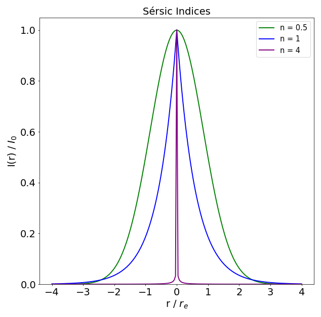
Sérsic Index
A Sérsic index determines the degree of curvature of the profile. The larger values of \(n\) get, the more concentrated the profile is at smaller radii. As \(n\) gets larger, the Sérsic model tends to a power-law with a slope equal to 5. n = 4 corresponds to a de Vaucouleurs’ profile which describes elliptical galaxies and the cores of spirals well; while n = 1 gives the exponential profile, which models spiral disks well. n = 0.5 gives a low concentration profile (Gaussian)
that can be used to model intra-cluster glow in galaxy clusters (assuming an elliptical shape), and can be used as an alternative to a Ferrer Profile.
Effective Radius and Intensity
\(r_{e}\) is the effective radius or half-light radius which encloses half of the total flux of the galaxy and can be defined by the following expression:
\(L(\leq r_e) = \frac{1}{2}L(\leq \infty)\).
\(I_e\) is the intensity or flux exactly at \(r_{e}\) and can be defined as \(I_e = I(r_{e})\) and determines the amplitude of the profile. \(I_e\) can be related to the intensity at the center of the Sérsic profile (\(I_0 = I(r_0)\)) as follows:
\(I_e = \frac{I_0}{\exp\left\{b_n\right\}}\)
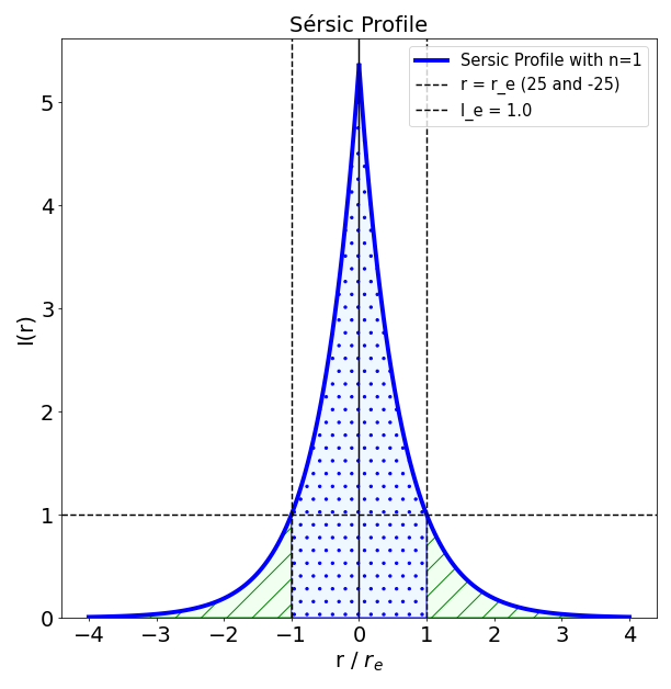
In this plot we see a one dimensional cross-section of a Sérsic Profile (arbitrary units) with \(r_e = 25\) and \(I_e = 1\). Notice how \(I_0\) is equal to 5.3 and not 1. The dotted blue area under the curve contains half of the total flux and is equal to the striped green area in value (the green area extends to infinity).
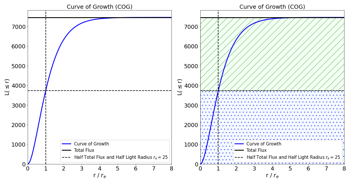
Curve of Growth
The curve of growth (COG) of a galaxy is the relationship between radius (from the galaxy center) and the total flux within that radius. It represents the cumulative flux enclosed at a given radius. The COG is very sensitive to background noise and fluctuations from the galaxy’s stochastic components. For a galaxy well described by a Sersic profile, the curve of growth is given by \(L(\leq r)\).
Below is a plot of the COG of a Sérsic profile with \((I_e=1, r_e=25, n=1)\):
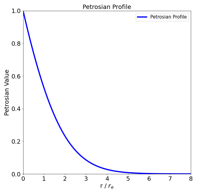
Petrosian Profiles
In petrofit, the Petrosian profile or Petrosian index \(\eta\) is defined as the inverse of the original formulation by Petrosian (1976), and has the property where \(\eta(0) = 1\) at the center of the galaxy and drops to zero at the edge:
\(\eta (r) = \frac{I(r)}{\langle I(r) \rangle} = I(r) \frac{A(r)}{L(\leq r)}\)
Where:
\(\eta (r)\) is the Petrosian at \(r\).
\(I(r)\) is the surface brightness at \(r\).
\(\langle I (r) \rangle\) is the average surface brightness within \(r\).
\(L(\leq r)\) is the total flux within \(r\).
\(A(r)\) is the aperture area. For elliptical apertures: \(A(r) = \pi \cdot (1 - ellip) \cdot r^2\)
Below is a plot Petrosian profile of a Sérsic model with \((I_e=1, r_e=25, n=1)\):
Discrete Computation
Given an array of enclosed fluxes (\(L\)) and corresponding aperture areas (\(A\)), the Petrosian profile can be computed discretely as follows:
Estimate the surface brightness by finding the average flux between the current index (\(i\)) and the last index (\(i-1\)). Note that the gap between apertures affects the accuracy of the surface brightness at \(i\), thus it is recommended to use apertures with radii that are incremented by a small number of pixels:
\begin{equation} I[i] \approx \frac {L[i] - L[i-1]} {A[i] - A[i-1]} \end{equation}
Estimate the average surface brightness by taking the flux at \(i\) and dividing it by the corresponding aperture area:
\begin{equation} {\langle I[i] \rangle} = \frac {L[i]} {A[i]} \end{equation}
Compute the Petrosian index at \(i\) using the estimated values in steps 1 and 2:
\begin{equation} \eta [i] = \frac{I[i]}{\langle I[i] \rangle} = \left(\frac {L[i] - L[i-1]} {A[i] - A[i-1]}\right) \cdot \frac {A[i]} {L[i]} \end{equation}
In discrete computations, the Petrosian profile can not be computed at the first index even if it corresponds to the center pixel (\(r[i_0]=0\)). In real images, the surface brightness of a galaxy is binned into pixels, and to accurately determine \(I_0\), one would need to infinitely oversample the central region. In other words, each pixel corresponds to a total surface brightness integrated within the area of the pixel as opposed to the surface brightness at the pixel coordinates. As
such, PetroFit sets the first Petrosian value to numpy.nan when returning a discretely computed array of Petrosian indices. PetroFit takes advantage of fact that the Petrosian index at the center of a galaxy is equal to \(1\) when computing radii internally.
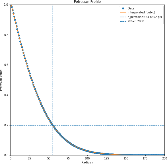
Petrosian Radius and Eta
The Petrosian radius is the radius at which the Petrosian profile is equal to a special Petrosian index \(\eta_{petro}\). In petrofit, the Petrosian radius is defined as the radius where \(\eta = 0.2\). Thus the Petrosian radius and \(\eta_{petro}\) (“eta”) can be defined as:
\(\eta( r_{petro} ) = \eta_{petro} = 0.2\)
Here is a plot of the Petrosian radius and \(\eta=0.2\) for a Sérsic profile with \((I_e=1, r_e=25, n=1)\):
Petrosian Total Flux Radius and Epsilon
The Petrosian total flux radius denotes the radius encompassing nearly all of a galaxy’s flux. Given the infinite nature of Sérsic profiles, a radius that encloses the entire flux isn’t feasible. Real galaxy images also include noise, making it impractical to measure minuscule flux values at vast radii. Consequently, within petrofit, the radius enclosing 99% of the galaxy’s light is termed the total flux radius.
This radius is defined by multiplying the Petrosian radius, \(r_{petro}\), with a constant known as epsilon (\(\epsilon\)), typically set to 2:
\(r_{total} = \epsilon \cdot r_{petro}\)
For various fractions of total luminosity, this concept can be generalized as:
\(r_{i} = \epsilon_{i} \cdot r_{petro}\)
Here, \(i\) represents the luminosity fraction: \(i = \frac{L(<r_i)}{L(<r_{total})}\).
Petrosian Half Light Radius
The Petrosian half-light radius is the radius which contains half of the total flux. This quantity is especially important because the half-light radius is equal to the Sérsic effective radius. The half-light radius can be computed by numerically finding the radius that encloses half of the total flux. Consequently, the Petrosian half-light radius can be defined as the radius which satisfies the following expression:
\(L(\leq r_{50}) = \frac{1}{2} L(\leq r_{total} )\)
Concentration Index
The concentration index is the ratio of the radii containing a specified fraction of the total flux and can be generalized as follows:
\begin{equation} C_{i o} \equiv 5 \cdot log\left(\frac{r_{o}}{r_{i}}\right) \end{equation}
where \(r_o\) and \(r_i\) are the outer and inner radii, enclosing \(o\%\) and \(i\%\) percent of the total flux respectively. The concentration index is related to the profile shape and can be used as a proxy for morphology. Some commonly used concentration indices are \(C_{2080}\) and \(C_{5090}\):
\begin{equation} C_{2080} = 5 \cdot log\left(\frac{r_{80}}{r_{20}}\right) \end{equation}
\begin{equation} C_{5090} = 5 \cdot log\left(\frac{r_{90}}{r_{50}}\right) \end{equation}
\(C_{2080}\) correlates better with the Sérsic index (and epsilon). However, in the presence of image degradation, \(C_{5090}\) may be more immune from systematic effects.
Petrosian Concentration Index
We can define the Petrosian concentration of radii derived from Petrosian indices as:
\begin{equation} P_{i o} \equiv 5 \cdot log\left(\frac{r(\eta_{o})}{r(\eta_{i})}\right) \end{equation}
where \(r(\eta_{0})\) and \(r(\eta_{i})\) denote the outer and inner Petrosian radii. These correspond to \(\eta_{0}\) and \(\eta_{i}\) Petrosian indices respectively. The merit of this definition is its direct computability from the Petrosian profile, thereby circumventing the need for estimating radii using the curve of growth.
Furthermore, we introduce a Petrosian concentration index, \(P_{0502}\), as:
\begin{equation} P_{0502} = 5 \cdot log\left(\frac{r(\eta_{0.2})}{r(\eta_{0.5})}\right) = 5 \cdot log\left(\frac{r_{petro}}{r(\eta_{0.5})}\right) \end{equation}
One significant advantage of this approach is that we can compute the concentration without needing to know the total flux, which is a requirement for metrics like \(C_{2080}\). This makes it especially beneficial in cases where total flux might be ambiguous or hard to determine precisely.
Petrosian Corrections
Petrosian magnitudes are primarily independent of redshift, relying on the ratio of two surface brightnesses. Yet, morphological K-corrections stemming from changes in the profile are applicable. A significant advantage of Petrosian magnitudes over variable aperture photometry methods, like Kron magnitudes (Kron 1980), is the sole dependency of the Petrosian radius on the light contained within its boundaries, ensuring minimized random errors in \(r_{petro}\) measurements.
However, the light percentage captured within \(2 \times r_{petro}\) is profile-dependent. For instance, while 99% of light from an exponential profile \(n = 1\) is within this range, an \(r^{1/4}\) profile captures only 83.4% of the light (Graham et al. 2005). This discrepancy necessitates adjustments to \(r_{total}\) using the suitable epsilon (\(\epsilon\)) value. A relationship between the concentration index and \(\epsilon\) can be deduced by simulating Sérsic profiles.
In ideal Sérsic model images, unaffected by noise or PSF, the concentration index (C2080) versus epsilon plot would resemble:
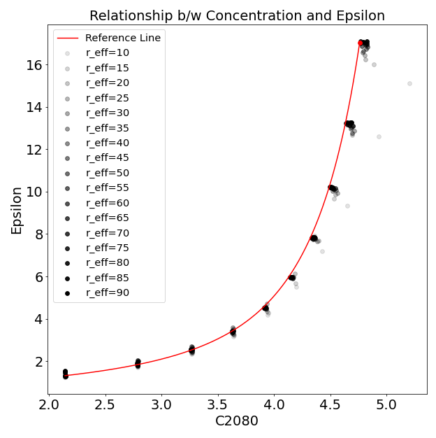
Higher concentration scatters are attributed to the model’s pixel grid sampling, particularly impacting profiles with small half-light radii and heightened concentrations due to a significant oversampling factor.
On the other hand, actual galaxy images incorporate noise and exhibit light smearing based on the instrument’s PSF, which reduces concentration and skews the previously derived relationship. An example plot showcases concentration indices of profiles, now convolved with the Hubble Space Telescope’s F105W PSF at 60 mas, alongside the earlier polynomial fit for comparison:
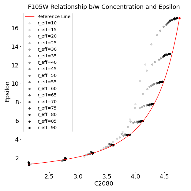
Especially for profiles with smaller half-light radii, PSF convolution introduces noticeable skews, underscoring the necessity for corrections that factor in both the half-light radius and PSF shape. For this reason, we must make corrections that account for the half-light radius and the shape of the PSF as well.
List of Galaxy Properties
The following galaxy properties can be computed using petrofit as described in this section:
Sersic Parameters
Petrosian Parameters
References
Bershady, M. A., Jangren, A., and Conselice, C. J., “Structural and Photometric Classification of Galaxies. I. Calibration Based on a Nearby Galaxy Sample”, The Astronomical Journal, vol. 119, no. 6, pp. 2645–2663, 2000. doi:10.1086/301386.
Crawford, S. M., “The distribution of star-forming galaxies in intermediate redshift galaxy clusters”, PhDT, 2006.
de Vaucouleurs, G. 1948, Annales d’Astrophysique, 11, 247
Graham, A. W., “Total Galaxy Magnitudes and Effective Radii from Petrosian Magnitudes and Radii”, The Astronomical Journal, vol. 130, no. 4, pp. 1535–1544, 2005. doi:10.1086/444475.
Graham, A. W. and Driver, S. P., “A Concise Reference to (Projected) Sérsic R1/n Quantities, Including Concentration, Profile Slopes, Petrosian Indices, and Kron Magnitudes”, Publications of the Astronomical Society of Australia, vol. 22, no. 2, pp. 118–127, 2005. doi:10.1071/AS05001.
Kent, S. M., “CCD Surface photometry of field galaxies.I. Observations.”, The Astrophysical Journal Supplement Series, vol. 56, pp. 105–141, 1984. doi:10.1086/190978.
Kron, R. G., “Photometry of a complete sample of faint galaxies.”, The Astrophysical Journal Supplement Series, vol. 43, pp. 305–325, 1980. doi:10.1086/190669.
Petrosian, V., “Surface Brightness and Evolution of Galaxies”, The Astrophysical Journal, vol. 210, p. L53, 1976. doi:10.1086/182301.
Sérsic, J. L. 1963, Boletin de la Asociacion Argentina de Astronomia La Plata Argentina, 6, 41 —. 1968, Atlas de Galaxias Australes