Galaxy Modeling
In this section, we demonstrate the basics of light profile modeling on a galaxy using a single component Sérsic profile. We also demonstrate how the photometry and petrosian PetroFit sub-models can be used to improve the initial guesses of the Sérsic parameters.
Please note that this is an extensive analysis to demonstrate PetroFit’s fitting workflow. Most practical applications of PetroFit will not require all of the steps discussed in this section.
To start with PetroFit, simply import it as follows:
[1]:
import petrofit as pf
Loading Example Data
The following data is a cutout of a group of bright galaxies in Abell 2744 (located at (3.596248, -30.388517)). The original data was acquired by the Hubble Frontier Fields team via the WFC3 instrument in the F105W filter and can be directly downloaded from the Mikulski Archive for Space Telescopes. The cutout image used
in this documentation can be found in the git repository at the following path petrofit/docs/data/abell_2744_dwarf_galaxy_f105w.fits.gz.
Loading Data and RMS Images
We first use astropy’s CCDData to load the example data and visualize it through matplotlib. The rms image is loaded using astropy’s fits sub-module.
[2]:
from astropy.nddata import CCDData
from astropy.io import fits

image = CCDData.read('data/abell_2744_dwarf_galaxy_f105w.fits.gz')
rms = fits.getdata('data/abell_2744_dwarf_galaxy_f105w_rms.fits.gz')
[4]:
import numpy as np
from matplotlib import pyplot as plt

plt.rcParams['figure.figsize'] = [6, 6]
plt.rcParams['image.origin'] = 'lower'
plt.rcParams['font.size'] = 12

vmax = 0.05 # Use the image std as max and min of all plots
vmin = - vmax

fig, axs = plt.subplots(1,2, figsize=[12, 6])
plt.sca(axs[0])
plt.imshow(image.data, vmin=vmin, vmax=vmax)
plt.title("Mock Galaxy")
plt.xlabel("Pixels")
plt.ylabel("Pixels")

plt.sca(axs[1])
plt.imshow(rms)
plt.title("RMS Image")
plt.xlabel("Pixels")
plt.ylabel("Pixels")
plt.show()
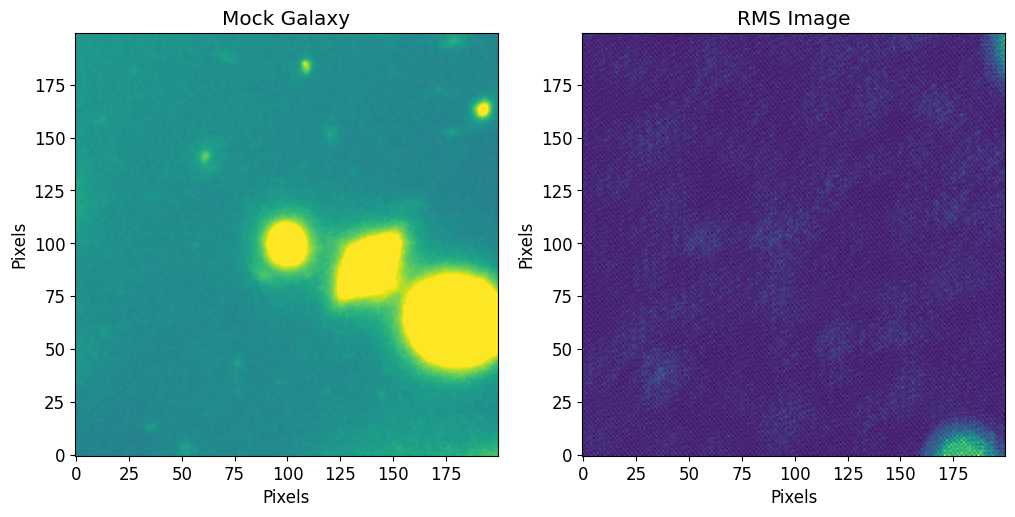
Image Errors
[5]:
from photutils.utils import calc_total_error
err = calc_total_error(
    data=image.data, # Input Image
    bkg_error=rms, # All sources of background error except source Poisson error
    effective_gain=image.header['EXPTIME'] # Factor to convert data units to counts
)
Make Source Catalog
We will use the sigma clipped std as a threshold at the segmentation and deblending steps.
[6]:
from astropy.stats import sigma_clipped_stats
image_mean, image_median, image_stddev = sigma_clipped_stats(image.data, sigma=3)
Here we identity sources in the input image.
[7]:
threshold = image_stddev * 3

# Min Source size (area)
npixels = 2**2

cat, segm, segm_deblend = pf.make_catalog(
    image.data,
    threshold=threshold,
    deblend=True,
    npixels=npixels,
    contrast=0.00,
    plot=True, vmax=vmax, vmin=vmin,
    figsize=[12, 6]
)

plt.show()

# Display source properties
print("Num of Targets:", len(cat))
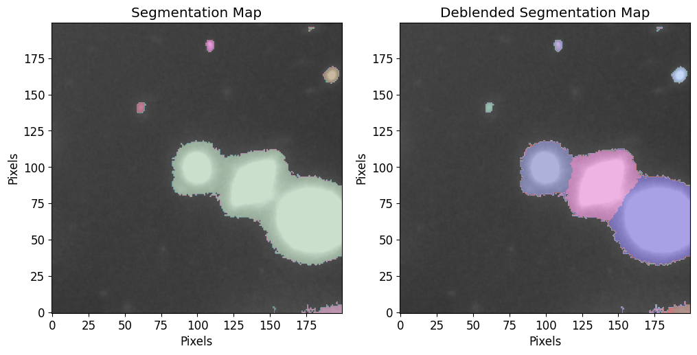
Num of Targets: 11
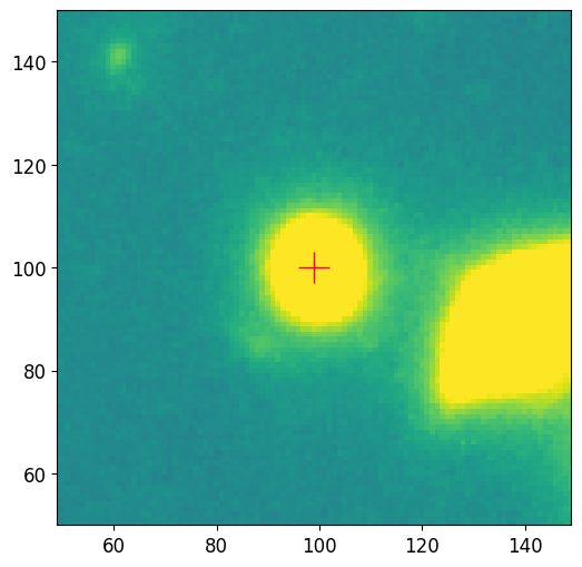
Single Source Photometry
Here we pick a galaxy that can be modeled using a single Sérsic model, the galaxy in the middle looks like an elliptical galaxy that can be well described by such a profile. To make sure we selected the right galaxy, we use the plot_target function to plot a cutout of the source.
[8]:
# Sort and select object of interest in the catalog
sorted_idx_list = pf.order_cat(cat, key='area', reverse=True)
idx = sorted_idx_list[2] # index 0 is largest
source = cat[idx]  # get source from the catalog

pf.plot_target(
    position=(source.maxval_xindex, source.maxval_yindex),
    image=image.data,
    size=100,
    vmax=vmax,
    vmin=vmin
)
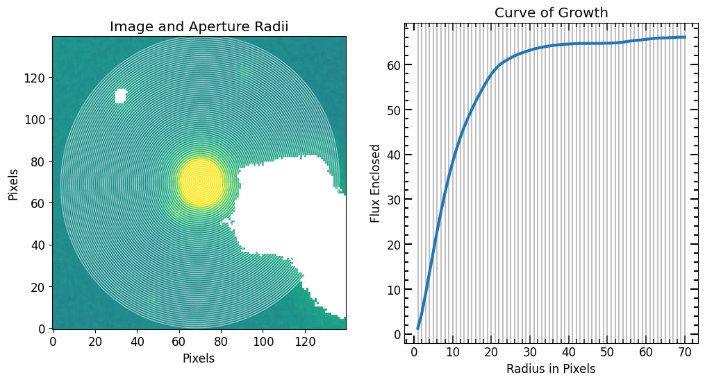
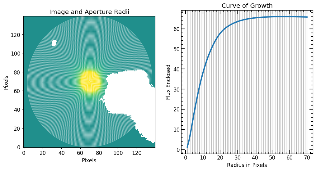
After selecting the source, we define a radius list for the aperture photometry. Once r_list is defined, we run the source_photometry step.
[9]:
# Max aperture radius
max_pix = 70

r_list = pf.make_radius_list(
    max_pix=max_pix, # Max pixel to go up to
    n=max_pix # the number of radii to produce (i.e 1 aperture per pixel increase in r)
)

print("len(r_list) = {}".format(len(r_list)))


# Photomerty
flux_arr, area_arr, error_arr = pf.source_photometry(
    # Inputs
    source, # Source (`photutils.segmentation.catalog.SourceCatalog`)
    image.data, # Image as 2D array
    segm_deblend, # Deblended segmentation map of image
    r_list, # list of aperture radii

    # Options
    error=err, # Error image (optional)
    cutout_size=max(r_list)*2, # Cutout out size, set to double the max radius
    bg_sub=True, # Subtract background
    sigma=3, sigma_type='clip', # Fit a 2D plane to pixels within 3 sigma of the mean
    plot=True, vmax=vmax, vmin=vmin, # Show plot with max and min defined above
)
plt.show()
len(r_list) = 70
11
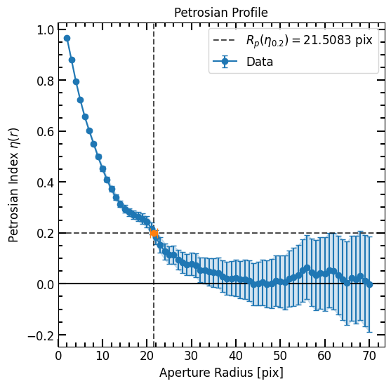
Petrosian Profile
We use the photometry that we obtained to construct a Petrosian profile of the galaxy. This will allow us to estimate the parameters of the galaxies Sérsic profile. We also initialize a PetrosianCorrection which we can use to estimate the Sérsic index (n) and r_eff (half-light radius). The correction grid we use for PetrosianCorrection was created specifically for this dataset using the PSF above.
[10]:
p = pf.Petrosian(r_list, area_arr, flux_arr, flux_err=error_arr)

pc = pf.PetrosianCorrection.read("data/f105w_psf_corr.ecsv")
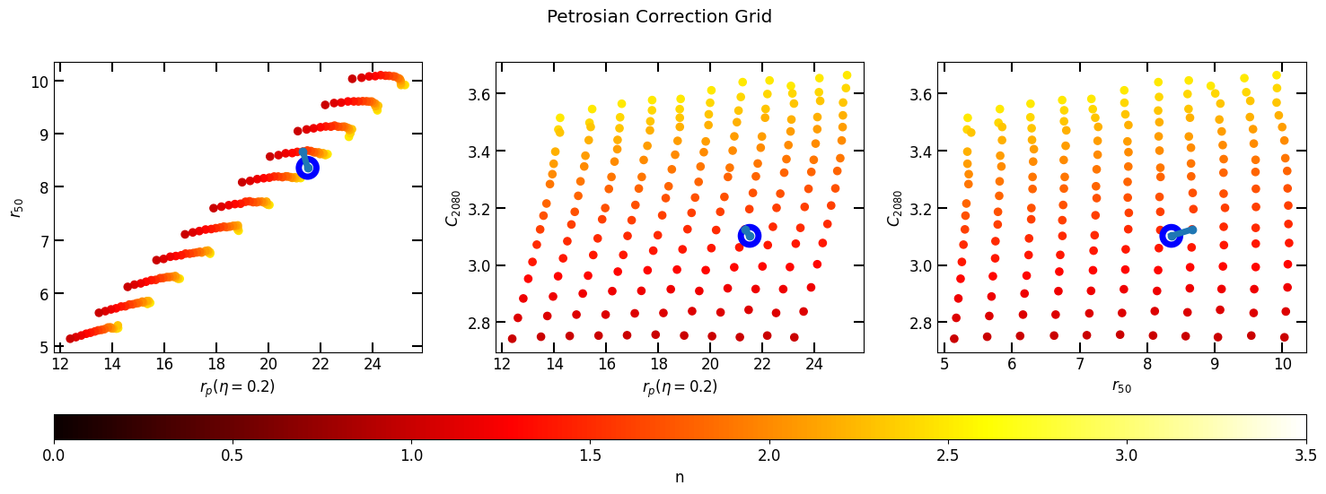
Next we compute and apply the epsilon that produces the correct r_total_flux and creates a new corrected Petrosian profile (corrected_p).
[11]:
pc.plot_correction(p)
plt.show()
corrected_p = pc.correct(p)
Galaxies with a high Sérsic index (high concentration) have r_total_fluxs that extend much further than we can possibly measure. If the corrected r_total_flux is out of the photometric range (i.e r_total_flux > max_pix), we would be unable to measure the flux at r_total_flux (the total flux), which also means that we would be unable to measure the Petrosian radius (np.nan is returned). If the corrected r_total_flux is out of range and we feel like the photometry data
range goes far out enough to estimate the total flux, we can set epsilon to a value that will result in a r_total_flux equal to the last photometry radius.
[12]:
max_photometry_r =  max(corrected_p.r_list)

if corrected_p.r_total_flux > max_photometry_r:
    print("Truncation was applied")
    truncated_epsilon = max_photometry_r / corrected_p.r_petrosian
    corrected_p.epsilon = truncated_epsilon
else:
    print("Truncation was not needed")

# Print Radii
print('total_flux = ', corrected_p.total_flux)
print('max_photometry_r = ', max_photometry_r)

# Plot Petrosian
corrected_p.plot()
plt.show()
Truncation was not needed
total_flux =  64.70574811498224
max_photometry_r =  70.0
Estimating Sérsic Parameters
astropy’s Sersic2D implements this model and allows us to provide initial guesses for the Sérsic parameters. Getting good estimates of these parameters is very important because the Levenberg-Marquardt algorithm is sensitive and may return parameters that correspond to a local minimum. Because of this, we follow the steps below to estimate the Sérsic parameters.
The Sersic2D model has the following parameters:
Center Pixel
We can use the get_source_position to find the max pixel position of the source in the image using the SourceCatalog object. Since this center is relative to the image, we save the result in image_x_0 and image_y_0.
Note
The x_0 and y_0 vlaues we use in the model in this example are defined in the Zoom and Mask Image section. This is because we make a cutout of the target at (image_x_0, image_y_0) which shifts the coordinate space. If no cutouts are made, then we can use (image_x_0, image_y_0) as the center of the astropy model.
[13]:
image_x_0, image_y_0 = pf.get_source_position(source)

print(image_x_0, image_y_0)
99 100
Ellipticity and Elongation
We pass the source’s SourceCatalog object to the get_source_ellip and get_source_elong functions to find the source’s light profile ellipticity and elongation respectively. These values are derived from the segmentation footprint of the source.
[14]:
ellip = pf.get_source_ellip(source)
elong = pf.get_source_elong(source)

print(ellip)
print(elong)
0.05500697093115503
1.0582088642340108
Source Orientation
We pass the source’s SourceCatalog object to the get_source_theta function to find the orientation of the light profile in radians, counterclockwise from the positive x-axis. In some catalogs, this value is known as the position angle.
[15]:
theta = pf.get_source_theta(source)

print(theta)
1.3370665448102104
Sérsic Index
The PetroFit PetrosianCorrection contains a grid that maps the uncorrected (PSF convolved) Petrosian half-light radius and concentration index to an epsilon value that gives the correct Petrosian radii. This grid can also be used to map the Petrosian radius, uncorrected half-light radius, and concentration index to a Sérsic index.
[16]:
n = pc.estimate_n(p)

print(n)
1.5
Half-Light Radius (r_eff)
We use the corrected Petrosian radius to estimate the half-light radius (r_eff).
[17]:
r_eff = corrected_p.r_half_light

print(r_eff)
8.356871374274856
Amplitude at r_eff
To find the flux at the half-light radius, we fit an elliptical isophote at r_eff using photutils’s Ellipse model using the get_amplitude_at_r function. If this value can not be computed, np.nan is returned so make sure to check using np.isnan(amplitude)
from photutils.isophote import EllipseGeometry, Ellipse

# Define EllipseGeometry using ellip and theta
g = EllipseGeometry(image_x_0, image_y_0, 1., ellip, theta)

# Create Ellipse model
ellipse = Ellipse(image.data, geometry=g)

# Fit isophote at r_eff
iso = ellipse.fit_isophote(r_eff)

# Get flux at r_eff
amplitude = iso.intens
[18]:
from petrofit.segmentation import get_amplitude_at_r
amplitude = get_amplitude_at_r(r_eff, image, image_x_0, image_y_0, ellip, theta)

print(amplitude)
0.07358068039517286
Zoom and Mask Image
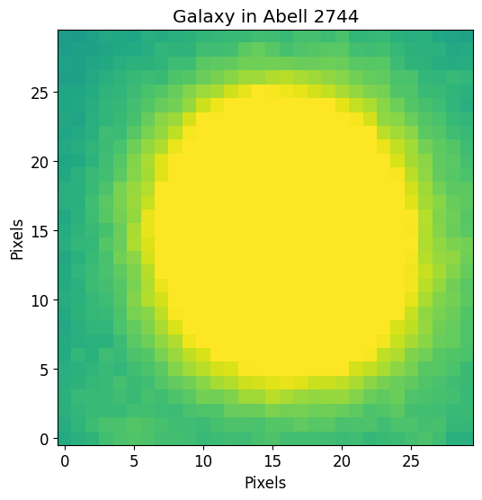
Before we fit the image, it is important to mask all nearby sources to avoid interference and zoom in to avoid fitting irrelevant pixels (especially those outside of r_total_flux). For this example, we will mask nearby sources using the masked_segm_image function that masks pixels using source segmentation footprints and make a zoomed cutout using astropy’s Cutout2D function. We also make a second cutout (fitting_image_unmasked) of the same dimensions as the fitting image,
but without masking nearby sources. We will subtract the fitted model from this unmasked image once the fitting is complete.
We make a cutout of size cutout_size centered at the source, as we identified in the finding center section, and define a new center (x_0 and y_0) that we will use in the astropy model.
[19]:
from astropy.nddata import Cutout2D

# Define cutout size
cutout_size = 30

# Make an image with all sources masked except `source`
masked_image = pf.masked_segm_image(source, image.data, segm_deblend, fill=None, mask_background=False)

# Make cutouts
fitting_image = Cutout2D(masked_image, (image_x_0, image_y_0), cutout_size, mode='partial', copy=True)
fitting_image_unmasked = Cutout2D(image.data, (image_x_0, image_y_0), cutout_size, mode='partial', copy=True)

# Define new center
x_0 = y_0 = cutout_size / 2

# Plot cutout that will be fit
plt.imshow(fitting_image.data, vmin=vmin, vmax=vmax)
plt.title("Galaxy in Abell 2744")
plt.xlabel("Pixels")
plt.ylabel("Pixels")
plt.show()
Make Sérsic Model
Astropy Model
[20]:
from astropy.modeling import models

center_slack = 4

sersic_model = models.Sersic2D(

        amplitude=amplitude,
        r_eff=r_eff,
        n=n,
        x_0=x_0,
        y_0=y_0,
        ellip=ellip,
        theta=theta,

        bounds = pf.get_default_sersic_bounds({
            'x_0': (x_0 - center_slack/2, x_0 + center_slack/2),
            'y_0': (y_0 - center_slack/2, y_0 + center_slack/2),
        }),
)
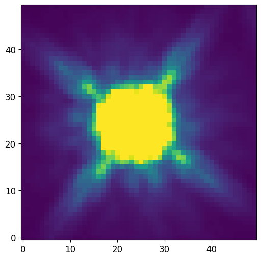
Load PSF
[21]:
from astropy.io import fits

# Load PSF image (2D array)
PSF = fits.getdata('data/f105w_psf.fits.gz')

# Normalize PSF
PSF = PSF / PSF.sum()

# Note that the PSF shape is odd on all sides
print("PSF Shape = {}".format(PSF.shape))

# Plot PSF and use vmax and vmin to show difraction spikes
plt.imshow(PSF, vmin=0, vmax=PSF.std()/10)
plt.show()
PSF Shape = (50, 50)
Oversampling
Oversample Entire Model Image
To oversample the image by a factor, you can pass a single integer value. For example:
[22]:
# Oversample the entire image by a factor of 5
oversample = 5
Create PetroFit Model
[23]:
psf_sersic_model = pf.PSFConvolvedModel2D(sersic_model, psf=PSF, oversample=oversample)
[24]:
# Disable the PSF rotation,
psf_sersic_model.fixed['psf_pa'] = True
Fitting the PSF Model
[25]:
fitting_err =  Cutout2D(err, (image_x_0, image_y_0), cutout_size, mode='partial', copy=True)
fitting_weights = 1 / fitting_err.data
To fit the galaxy we prepared with the PSFConvolvedModel2D we constructed, we call the fit_model as follows:
[26]:
%%time

from astropy.modeling import fitting
fitted_model, fit_info = pf.fit_model(
    fitting_image.data, psf_sersic_model,
    weights=fitting_weights,
    calc_uncertainties=True,
    maxiter=10000,
    epsilon=1.4901161193847656e-08,
    acc=1e-09,
)
CPU times: user 99.8 ms, sys: 982 μs, total: 101 ms
Wall time: 101 ms
[27]:
pf.print_model_params(fitted_model)
0.0817  amplitude
7.9921  r_eff
1.6808  n
15.9168 x_0
14.4015 y_0
0.1147  ellip
1.9610  theta
0.0000  psf_pa
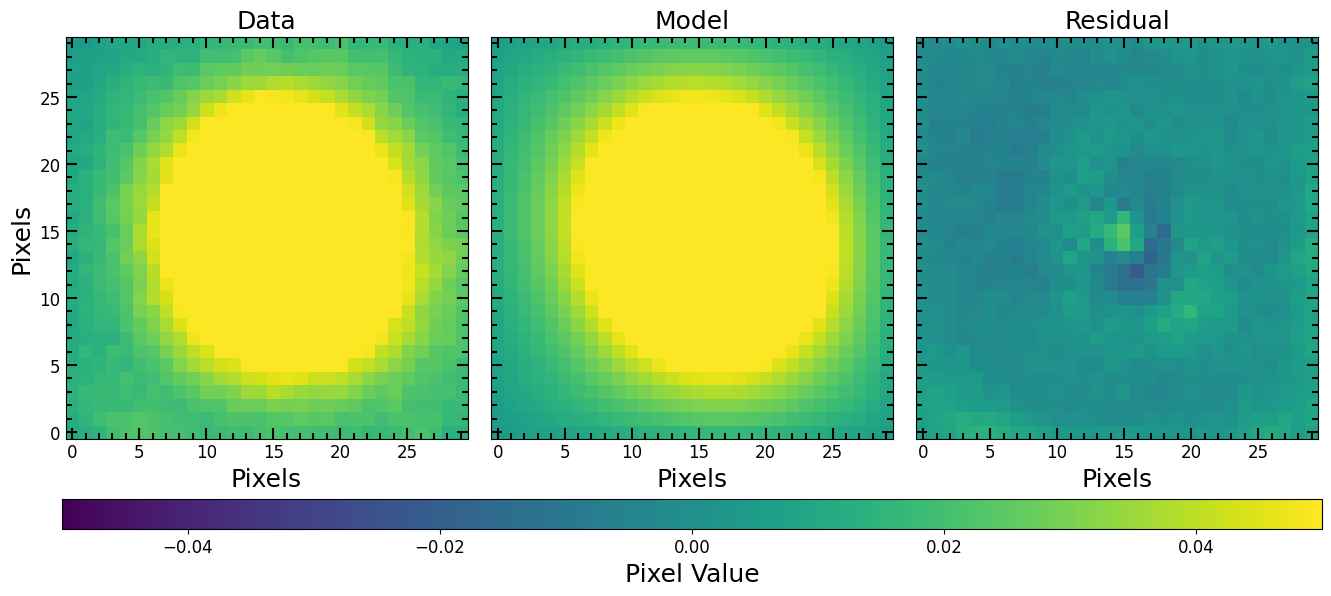
Model Visualization
[28]:
pf.plot_fit(fitted_model, fitting_image_unmasked, vmax=vmax, vmin=vmin, figsize=[3*6, 6])
plt.show()
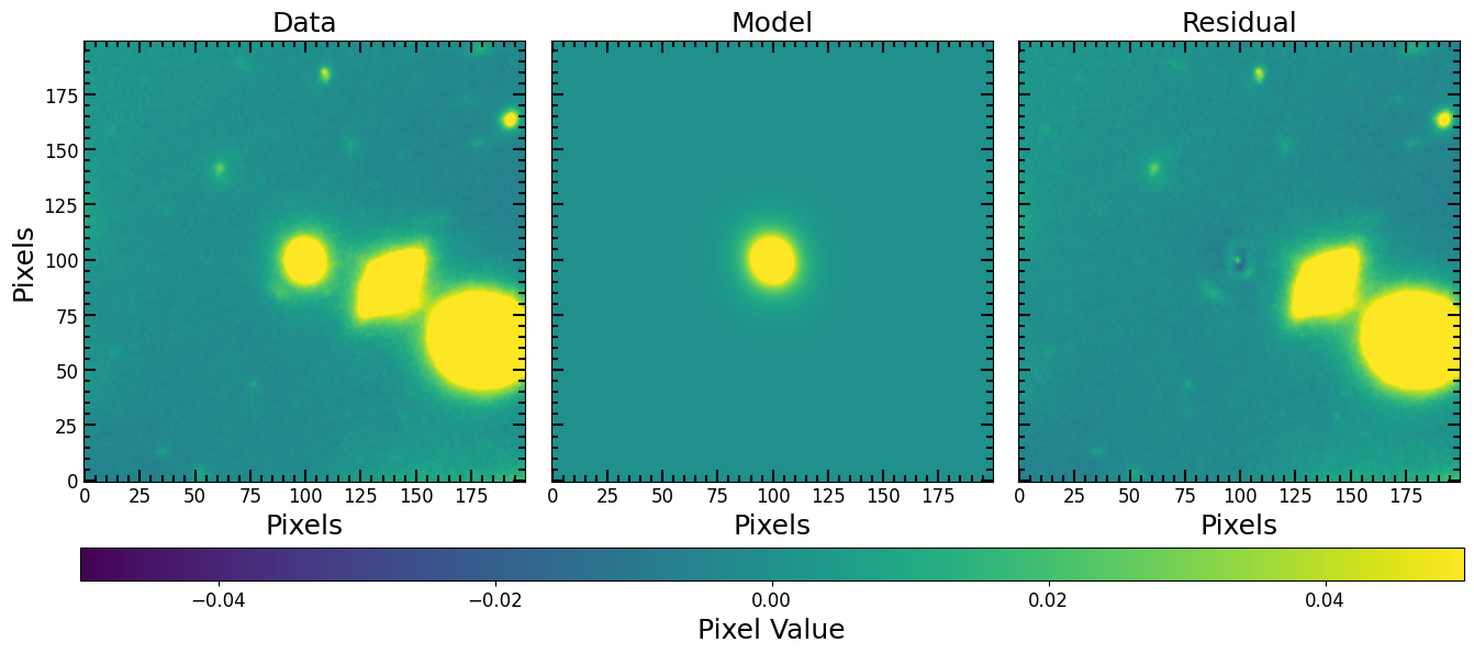
If we want to make a model image that we can subtract from the original data image, we just update the center of the model and generate a model image the same dimensions as the original image.
[29]:
from copy import deepcopy

# Reposition the Model
# --------------------

# Copy the model before changing the parameters
fitted_model_copy = deepcopy(fitted_model)

# Change the frame of reference from the fitting
# image to the original data coordinates.
# Remember that (x_0, y_0) -> (image_x_0, image_y_0)
fitted_model_copy.x_0 =  image_x_0 + (fitted_model.x_0 - x_0)
fitted_model_copy.y_0 =  image_y_0 + (fitted_model.y_0 - y_0)

# Make Model Image
# ----------------

# Set the size of the model image equal to the original image
full_fitted_image_size = image.data.shape[0]

# Center the model image at the center of the original image
# so the two images cover the same window
full_fitted_image_center = full_fitted_image_size // 2

# Generate a model image from the model
full_fitted_model_image = pf.model_to_image(
    fitted_model_copy,
    full_fitted_image_size,

)

# Plot Model Image
# ----------------
pf.plot_fit(fitted_model_copy, image.data,vmin=vmin, vmax=vmax)
plt.show()
Estimated vs. Fitted Parameters
In this section we compare the initial estimates that we derived purely from photometry vs. the parameters that were fit to the data. In the printout below, we see the fitted values in the first column and our initial guesses in the second column for each parameter.
[30]:
assumptions = [
    amplitude,
    r_eff,
    n,
    x_0,
    y_0,
    ellip,
    theta,
    0 # psf_pa
]

param_stds = fitted_model.stds

print("assum\tfit\t\tparam_name")
for param_name, param_val, param_std, assumption in zip(fitted_model.param_names, fitted_model.parameters,  param_stds.stds, assumptions):
    print("{:0.2f}\t{:0.2f} ± {:0.3f}\t{}".format(assumption, param_val, param_std, param_name))
assum   fit             param_name
0.07    0.08 ± 0.001    amplitude
8.36    7.99 ± 0.048    r_eff
1.50    1.68 ± 0.013    n
15.00   15.92 ± 0.006   x_0
15.00   14.40 ± 0.007   y_0
0.06    0.11 ± 0.003    ellip
1.34    1.96 ± 0.013    theta
Galaxy vs. Model Profiles
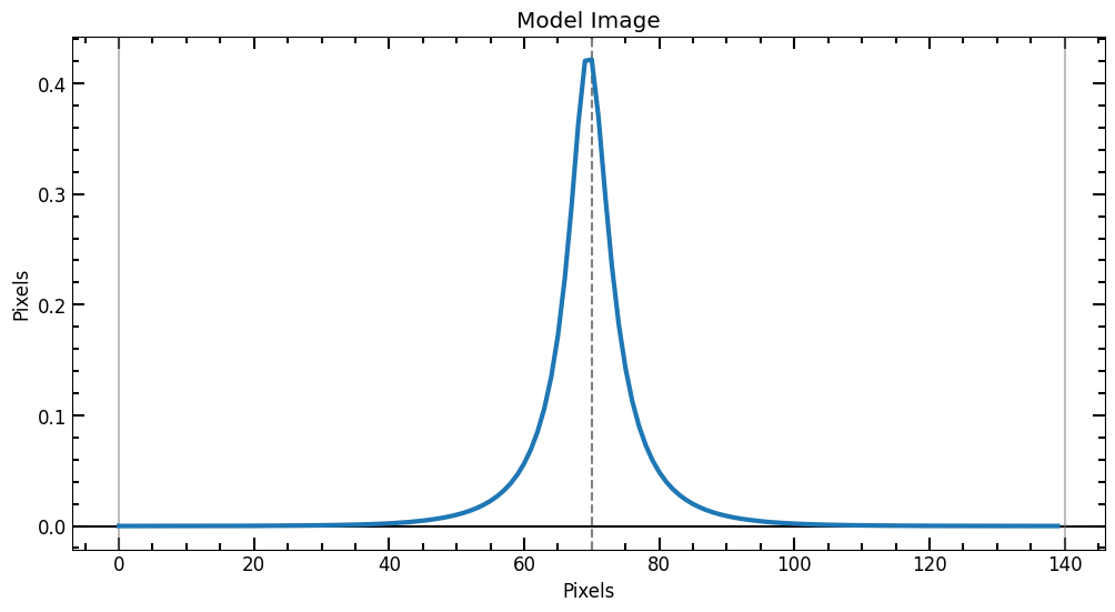
Now that we have a model image, we can do photometry and compare the Petrosian measurements of the model to that of the original galaxy image. Since we know the exact position of the target in the model image and because there are no intruding sources, we can perform direct photometry using photometry_step function.
[31]:
# Photomerty
model_flux_arr, model_area_arr, model_error_arr = pf.source_photometry(

    # Inputs
    source, # Source (`photutils.segmentation.catalog.SourceCatalog`)
    full_fitted_model_image, # Image as 2D array
    segm_deblend, # Deblended segmentation map of image
    r_list, # list of aperture radii

    # Options
    cutout_size=max(r_list)*2, # Cutout out size, set to double the max radius
    bg_sub=True, # Subtract background
    sigma=3, sigma_type='clip', # Fit a 2D plane to pixels within 3 sigma of the mean
    plot=True, vmax=vmax, vmin=vmin, # Show plot with max and min defined above
)

plt.title("Model Image")
plt.xlabel("Pixels")
plt.ylabel("Pixels")
plt.show()
11
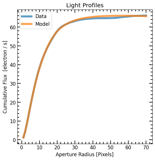
[32]:
# Plot Light profile
plt.plot(r_list, flux_arr, label='Data', lw=5, alpha=0.7)
plt.plot(r_list, model_flux_arr, label='Model', lw=5, alpha=0.7)

plt.title("Light Profiles")
plt.xlabel("Aperture Radius [Pixels]")
plt.ylabel("Cumulative Flux  [{}]".format(image.unit))
pf.mpl_tick_frame()
plt.legend()
plt.show()
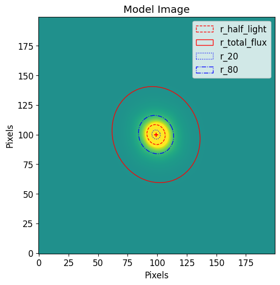
Petrosian Radii Comparison
We compare the Petrosian profiles and radii of the two images.
[33]:
model_p = pf.Petrosian(r_list, model_area_arr, model_flux_arr)

model_corrected_p = pc.correct(model_p)


# Plot Image
plt.imshow(full_fitted_model_image, vmax=vmax, vmin=vmin)

model_position = (
    fitted_model_copy.x_0.value,
    fitted_model_copy.y_0.value)

model_position = (image_x_0, image_y_0)
model_elong = 1 / (1 - fitted_model_copy.ellip.value)

model_theta = fitted_model_copy.theta.value

model_corrected_p.imshow(
    position=model_position,
    elong=model_elong,
    theta=model_theta
)

plt.title("Model Image")
plt.xlabel("Pixels")
plt.ylabel("Pixels")
plt.legend()
plt.show()
[34]:
corrected_p.plot(plot_r=True)
model_corrected_p.plot(plot_r=True, color='tab:orange')

plt.gca().get_legend().remove()
plt.show()
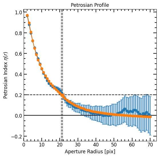
[35]:
print("Data r_total_flux = {:0.2f}".format(corrected_p.r_total_flux))
print("Model r_total_flux = {:0.2f}".format(model_corrected_p.r_total_flux))
Data r_total_flux = 42.44
Model r_total_flux = 41.22
[36]:
print("Data r_half_light = {:0.2f}".format(corrected_p.r_half_light))
print("Model r_half_light= {:0.2f}".format(model_corrected_p.r_half_light))
Data r_half_light = 8.36
Model r_half_light= 8.54
Total Flux Comparison
Finally we compare the total Petrosian flux of the data vs the model:
[37]:
print("Data Corrected Total Flux = {:0.2f}".format(corrected_p.total_flux * image.unit))
print("Model Corrected Total Flux = {:0.2f}".format(model_corrected_p.total_flux * image.unit))
Data Corrected Total Flux = 64.71 electron / s
Model Corrected Total Flux = 65.50 electron / s
[38]:
print("Data Corrected AB mag = {:0.2f} mag".format(pf.hst_flux_to_abmag(corrected_p.total_flux, image.header) ))
print("Model Corrected AB mag = {:0.2f} mag".format(pf.hst_flux_to_abmag(model_corrected_p.total_flux, image.header) ))
Data Corrected AB mag = 21.74 mag
Model Corrected AB mag = 21.73 mag