Petrosian
In this section, we use the photometric measurements (curve of growth) that were made in the Photometry section to construct a Petrosian profile. We use the Petrosian profile to measure various radii and concentrations. For a quick guide on how to construct curves of growth and Petrosian profiles, please see the Making a Photutils Source Catalog and Curve of Growth and Petrosian Radii sections in the Quick Start guide.
To start with PetroFit, simply import it as follows:
[1]:
import petrofit as pf
Loading Example Data
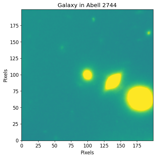
The following data is a cutout of a group of bright galaxies in Abell 2744 (located at (3.596248, -30.388517)). The original data was acquired by the Hubble Frontier Fields team via the WFC3 instrument in the F105W filter and can be directly downloaded from the Mikulski Archive for Space Telescopes. The cutout image used
in this documentation can be found in the git repository at the following path petrofit/docs/data/abell_2744_dwarf_galaxy_f105w.fits.gz.
We first use astropy’s CCDData to load the example data and visualize it through matplotlib.
[2]:
from astropy.nddata import CCDData
from astropy.io import fits

image = CCDData.read('data/abell_2744_dwarf_galaxy_f105w.fits.gz')
rms = fits.getdata('data/abell_2744_dwarf_galaxy_f105w_rms.fits.gz')
[4]:
from matplotlib import pyplot as plt

plt.rcParams['figure.figsize'] = [6, 6]
plt.rcParams['image.origin'] = 'lower'
plt.rcParams['font.size'] = 12

vmax = image.data.std() # Use the image std as max and min of all plots
vmin = - vmax

plt.imshow(image.data, vmin=vmin, vmax=vmax)
plt.title("Galaxy in Abell 2744")
plt.xlabel("Pixels")
plt.ylabel("Pixels")
plt.show()
Load Photometry
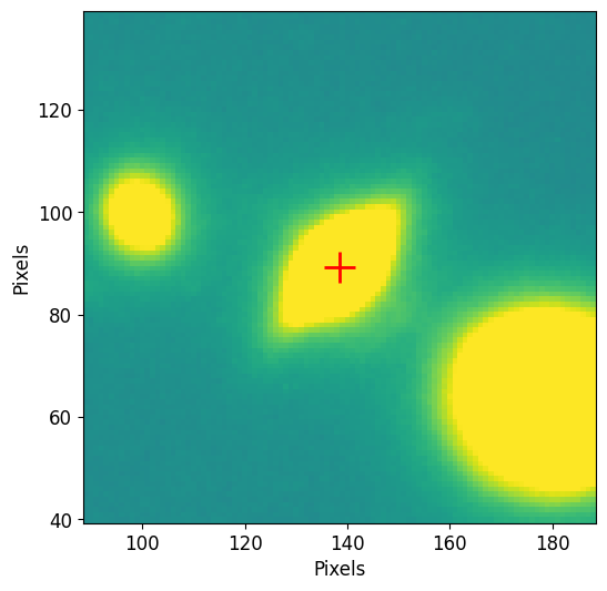
In the Photometry Chapter we constructed a curve of growth for the football shaped galaxy displayed there:
[5]:
pf.plot_target(image.data, (138.5, 89.3), size=100,
               vmin=vmin, vmax=vmax, lw=2)
plt.xlabel("Pixels")
plt.ylabel("Pixels")
plt.show()
We load the photometry as follows:
[6]:
import numpy as np
from astropy.table import Table
phot_table = Table.read('data/abell_2744_galaxy_f105w_photometry.ecsv') # Read table

# Load data
r_list = np.array(phot_table['r_list'])
flux_arr = np.array(phot_table['flux_arr'])
area_arr = np.array(phot_table['area_arr'])
error_arr = np.array(phot_table['error_arr'])
Construct Petrosian from Photometry
In this section, we use photometric values stored in flux, aperture area, and radii arrays to construct a Petrosian object. The following inputs are needed as inputs:
r_list: Array of radii in pixels.area_list: Array of aperture areas.flux_list: Array of photometric flux values within apertures.error_arr: Array of flux errors.
These values should represent the curve of growth and can be computed by using the PetroFit photometry tools.
We can also specify the eta and epsilon values.
eta(default=0.2) is the Petrosian value that defines the Petrosian radius.epsilon(default=2) is used to determine the radius of total flux.r_total_flux = r_petrosian * epsilon
[7]:
p = pf.Petrosian(r_list, area_arr, flux_arr, flux_err=error_arr)
Petrosian Radii
PetroFit uses the curve of growth of a galaxy’s flux to compute its Petrosian properties such as Petrosian radius and concentration index.
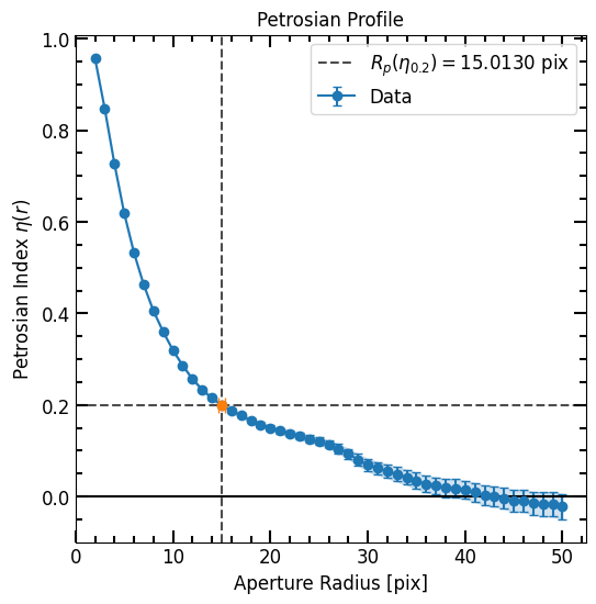
Petrosian Radius
The Petrosian radius is defined as the radius at which the Petrosian profile reaches the Eta (eta, default=0.2) value.
[8]:
print("{:0.4f} ± {:0.4f} pix".format(p.r_petrosian, p.r_petrosian_err))
15.0130 ± 0.2901 pix
Petrosian Total Flux Radius
The Petrosian flux or total flux radius is the radius that ideally encloses all the flux of the galaxy. The Petrosian total flux radius is estimated by multiplying r_petrosian with epsilon (default=2).
r_total_flux = r_petrosian * epsilon
We can use the r_total_flux_arcsec function, by passing it a WCS object, to compute the total flux radius in arcsec.
[9]:
print("{:0.4f} ± {:0.4f} pix".format(p.r_total_flux, p.r_total_flux_err))
30.0236 ± 0.5881 pix
[10]:
p.r_total_flux_arcsec(image.wcs) # arcsec
[10]:
np.float64(1.8014159492850954)
Petrosian Half-Light Radius
The half-light radius contains half of the galaxy’s total flux. To compute the half-light radius, we find the total flux (flux at r_total_flux) and divide it by half to find the “half flux” or “half-light”. We then find the pixel closest to the half-light value and define it as the half-light radius. Please note that interpolation is used between the input flux radii to find the radius that best matches the half-light flux.
We can use the r_half_light_arcsec function, by passing it a WCS object, to compute the half-light radius in arcsec.
[11]:
print("{:0.4f} ± {:0.4f} pix".format(p.r_half_light, p.r_half_light_err))
6.3617 ± 0.0245 pix
[12]:
p.r_half_light_arcsec(image.wcs) # arcsec
[12]:
np.float64(0.3817002693031062)
Fraction of Flux Radius
We can compute a radius that contains a specific fraction of the total flux using the fraction_flux_to_r function. For example we can compute the radius that contains 60% of the total flux as follows:
[13]:
r_60 = p.fraction_flux_to_r(fraction=0.6) # pixels
r_60_err = p.fraction_flux_to_r_err(fraction=0.6) # pixels
print("{:0.4f} ± {:0.4f} pix".format(r_60, r_60_err))
8.0378 ± 0.0343 pix
Concentration Index
The concentration index is the ratio of two aperture radii that contain a fraction (percent) of the total flux. It is computed as follows
concentration_index = 5 * np.log10( r(fraction_2) / r(fraction_1) )
The default is set to fraction_1 = 0.2 and fraction_2 = 0.8. The concentration_index function returns the r_fraction_1, r_fraction_2 and concentration_index.
In these examples, we comput the default C2080 and C5090 concentration indices for the input galaxy:
[14]:
r_20, r_80, c2080 = p.concentration_index()  # defualt c2080

r_20, r_80, c2080 # Radii in pixels
[14]:
(np.float64(2.891778355671134),
 np.float64(13.693538707741547),
 np.float64(3.376753454810066))
[15]:
r_50, r_90, c5090 = p.concentration_index(
    fraction_1=0.5,
    fraction_2=0.9
)

r_50, r_90, c5090 # Radii in pixels
[15]:
(np.float64(6.361672334466893),
 np.float64(19.349269853970792),
 np.float64(2.4154664252033426))
Total Petrosian Flux
We can also use Petrosian to compute the total Petrosian flux, which is defined as the flux at r_total_flux. If the r_total_flux is outside the photometric aperture radii, np.nan is returned.
[16]:
print("{:0.4f} ± {:0.4f} pix".format(p.total_flux, p.total_flux_err))
243.4296 ± 0.6000 pix
For Hubble data, we can use the flux_to_abmag function to convert flux values into mags by providing a header.
[17]:
pf.hst_flux_to_abmag(p.total_flux, header=image.header) # Mag
[17]:
np.float64(20.302884381698544)
Petrosian and COG Plots
Profile Plot
The Petrosian plot shows the Petrosian profile, the eta valued to define the Petrosian radius and the Petrosian radius.
[18]:
# Plot the Petrosian profile
p.plot()
plt.show()
Much in the same way we can plot the curve of growth as follows:
[19]:
# Plot curve of growth
p.plot_cog(flux_unit=image.unit)

plt.show()
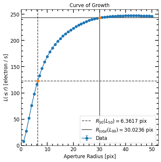
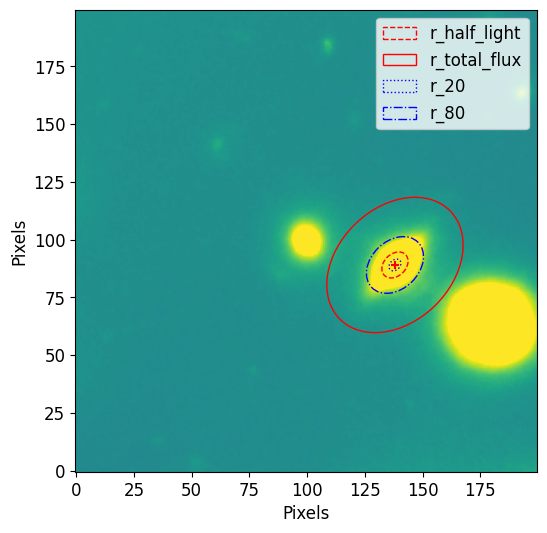
Image Overplot
Another way to visualize the radii is to overplot them over an image. To do this we first plot the image as usual and use the Petrosian.imshow function to overplot the r_half_light, r_total_flux, r_20 and r_80. The Petrosian.imshow requires the center of the apertures and plots the radii in pixels. Since elliptical apertures were used, we also provide the elongation and orientation (theta) of the apertures. We get these values from the source object and use
utility functions (get_source_position, get_source_elong, get_source_theta) as showen in the Photometry section.
[20]:
position = phot_table.meta['position']
elong = phot_table.meta['elong']
theta = phot_table.meta['theta']

p.imshow(position=position, elong=elong, theta=theta, lw=1.25)

plt.imshow(image.data, vmax=vmax, vmin=vmin)
plt.xlabel("Pixels")
plt.ylabel("Pixels")
plt.legend()
plt.show()

Change eta and epsilon
We can change the Petrosian eta and epsilon values after the Petrosian object has been initiated by setting their respective attributes. After setting the attributes, all other calculations and plots will use the new values.
In this example we copy the Petrosian object and change the eta and epsilon values to see how the radii change. Note how r_half_light and r_total_flux changed. To review:
eta: The Petrosian index, which dictates the value at which the Petrosian radius is determined. Typically, the default value is 0.2.epsilon: A multiplication factor used to scale the Petrosian radius to compute the “epsilon radius” (r_epsilon). If epsilon is0.275, for instance, thenr_epsilonwould be0.275 * r_p.r_epsilon: Refers to the “epsilon radius”. It’s the radius that encompasses an epsilon_fraction of the galaxy’s total flux. This radius is derived from the Petrosian radius by scaling it with the epsilon factor:r_epsilon = epsilon * r_p.epsilon_fraction: Represents the fraction of the total flux contained within ther_epsilon. For instance, a value of 0.5 suggests that 50% of the galaxy’s total flux is inside this radius.
By default epsilon_fraction = total_flux_fraction = 0.99 or 0.98, therefore the defualt is r_epsilon = r_total_flux.
[21]:
from copy import copy

p_copy = copy(p)
p_copy.eta = 0.13
p_copy.epsilon = 0.275
p_copy.epsilon_fraction = 0.5

print('eta =', p_copy.eta)
print('epsilon =', p_copy.epsilon)
print('r_half_light (old vs new) = {:0.2f} vs {:0.2f}'.format(p.r_half_light, p_copy.r_half_light))
print('r_total_flux (old vs new) = {:0.2f} vs {:0.2f}'.format(p.r_total_flux, p_copy.r_total_flux))
eta = 0.13
epsilon = 0.275
r_half_light (old vs new) = 6.36 vs 6.41
r_total_flux (old vs new) = 30.02 vs 32.63
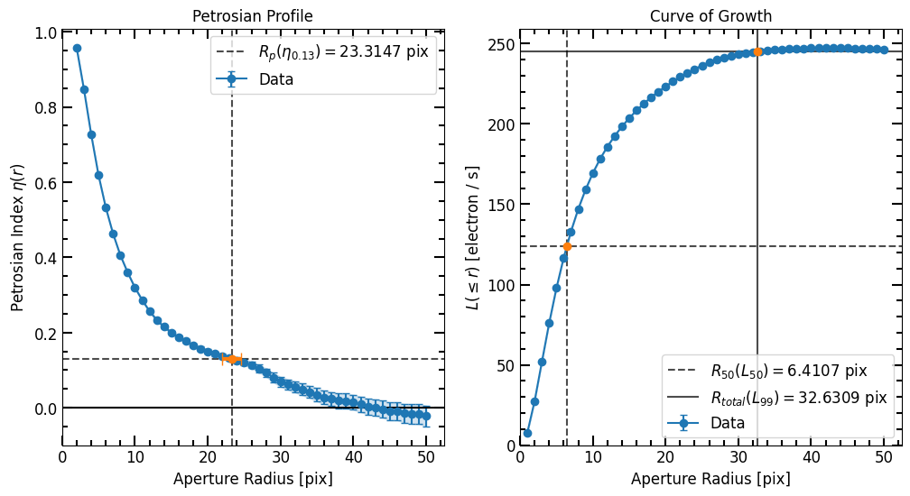
[22]:
# Plot
fig, axs = plt.subplots(1,2, figsize=(12, 6))
plt.sca(axs[0])
p_copy.plot(plot_r=True)

plt.sca(axs[1])
p_copy.plot_cog(plot_r=True, flux_unit=image.unit)

plt.show()
Corrections and Approximations
Important Note
Before going into corrections and approximations of Petrosian profiles, it’s important to understand the broader context in which they’re utilized. A significant portion of astronomical literature, including foundational analyses from the Sloan Digital Sky Survey (SDSS), predominantly relies on standard parameters: \(\eta=0.2\) and \(\epsilon=2\) for deriving the total flux. The rationale behind this prevalent practice is two-fold:
Noise Considerations: In real-world observations, the faint extremities of galaxies often lie beneath the instrument’s noise threshold. This can render intricate corrections superfluous since the adjustments might not significantly alter the results.
Practicality Over Precision: While the discussed corrections provide higher precision, their application demands optimal background subtraction. Hence, they’re often reserved for scenarios that have ideal subtraction for flux measurements or for measuring a galaxy’s size at higher precision given low signal-to-noise.
In other words, the default settings have historically been good enough. Given this backdrop, the forthcoming sub-section goes into specific techniques for those seeking to venture beyond the default parameters, either out of necessity or research specificity.
Techniques
For accurately determining the total flux, the epsilon value should ideally be a function of the Sérsic index. As the Sérsic index is correlated with the concentration index, we can leverage the measured concentration index to derive the appropriate value of epsilon, which, in turn, helps pinpoint the radii for total flux measurements.
To estimate epsilon, a few methods are at our disposal:
Utilizing Approximations:
Using the uncorrected concentration index (
U2080), we can approximate both the Sérsic index and the corrected epsilon. This method relies on approximations derived from fitting these relationships against a standard Sérsic profile.Pros:
A swift and straightforward means to approximate the Sérsic index and the corrected epsilon.
Only requires a moderate level of background subtraction.
Cons:
Does not account for PSF, which notably affects high Sérsic index profiles with a small \(r_{50}\).
Assumes an ideal singular Sérsic component profile (no noise limit). This could lead to a total flux radius that’s significantly larger than what is practically measurable.
[23]:
U2080 = p.c2080 # Uncorrected concentration index
C2080 = pf.PetroApprox.u2080_to_c2080(U2080) # Corrected concentration index
sersic_index = pf.PetroApprox.c2080_to_n(C2080) # Sersic index
corrected_epsilon = pf.PetroApprox.n_to_epsilon(sersic_index) # Corrected epsilon

# Correct:
p_approx = copy(p) # Copy
p_approx.epsilon = corrected_epsilon

print(corrected_epsilon)
2.7482732547874367
Adopting ``epsilon=0.5`` & ``epsilon_fraction=0.5``:
This method leverages the observation that for a wide range of Sérsic indices, the half-light radius (\(r_{50}\)) is approximately half of the Petrosian radius. This approximation is particularly helpful if our interest is primarily in determining \(r_{50}\) and if the curve of growth does not extend to the total flux radius of the uncorrected petrosian profile.
Pros:
Simplifies the process by using a consistent approximation across different Sérsic indices.
Does not require the curve of growth to extend to the total flux radius.
Can be faster and more direct when only \(r_{50}\) is of interest.
Cons:
Might not be the most accurate method for determining total flux or for profiles with significant deviations from the average. This is because the slope of the curve of growth is steep near \(r_{50}\).
Assumes the relationship between the half-light radius and petrosian radius is consistent across different galaxy profiles.
[24]:
# Correct:
p_r_50 = copy(p) # Copy
p_r_50.epsilon = 0.5  # epsilon
p_r_50.epsilon_fraction = 0.5 # epsilon corrsponds to 50% of total flux

print(p.r_50, p_approx.r_50, p_r_50.r_50)
6.361672334466893 6.479295859171834 7.508501700340068
This results in a \(r_{50}\) that is about a pixel off from the approximated and uncorrected profiles in this example. But the total flux radii will be poorly approximated by this method (~30% error):
[25]:
print(p.r_total_flux, p_approx.r_total_flux)
30.02360472094419 41.25665133026605
Utilizing Correction Grids:
This approach involves the simulation of a grid of Sérsic profiles, each varying in terms of Sérsic index and effective radius. This simulation results in a lookup table that associates the petrosian radius, the uncorrected half light radius, and the
C2080value with specific Sérsic index and corrected epsilon values.Pros:
Amongst available methods, this stands as the most precise, especially when focusing on single Sérsic component profiles.
Takes into account the PSF, which is important for high Sérsic index profiles due to it “smearing out” radii.
Cons:
Conducting simulations can be time-consuming.
Vastly different PSFs across multiple bands necessitate individual grids for each.
Effective corrections demand accurate image background subtraction.
Plese see the Correction Grids section for more details on how to generate correction grids.
[26]:
# Read F105W grid:
pc = pf.PetrosianCorrection.read('./data/f105w_psf_corr.ecsv')

# Pass uncorrected p to the correct function
p_corrected = pc.correct(p)

print(p.r_50, p_approx.r_50, p_r_50.r_50, p_corrected.r_50)
6.361672334466893 6.479295859171834 7.508501700340068 6.420484096819363
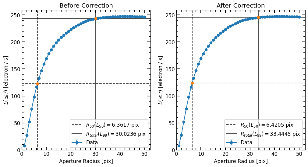
[27]:
# Plot
fig, axs = plt.subplots(1,2, figsize=(12, 6))
plt.sca(axs[0])
ax = p.plot_cog(plot_r=True, flux_unit=image.unit)
ax.set_title('Before Correction')

plt.sca(axs[1])
ax = p_corrected.plot_cog(plot_r=True, flux_unit=image.unit)
ax.set_title('After Correction')
plt.show()
[28]:
plt.imshow(image.data, vmax=vmax, vmin=vmin)
p_corrected.imshow(position=position, elong=elong, theta=theta)
plt.xlabel("Pixels")
plt.ylabel("Pixels")
plt.legend()
plt.show()