Image Fitting

Most galaxy light profiles can be well described by PSF convolved models like the Sérsic profile. PetroFit uses the astropy modeling sub-module to provide tools to perform two-dimensional fits of galaxy light profiles. To this end, we use the PetroFit PSFConvolvedModel2D class, which applies PSF convolution to and handles oversampling for astropy based models.

In this section, we demonstrate the basics of light profile modeling on a galaxy using a single component Sérsic profile.

To start with PetroFit, simply import it as follows:

import petrofit as pf

Loading Example Data

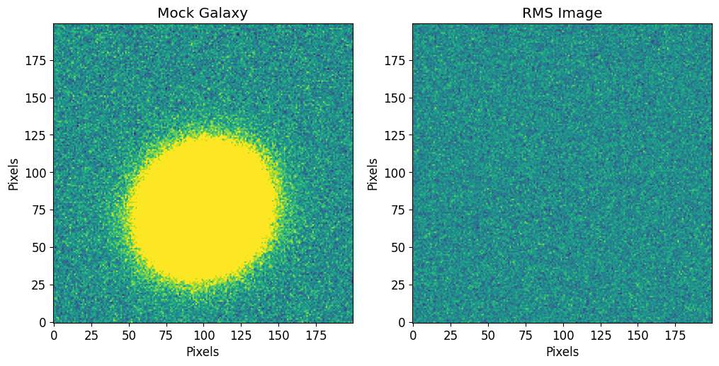
The dataset we’re using is a synthetic image of a galaxy, created using astropy’s Sersic2D model. This galaxy representation is convolved with a PSF for the F105W filter using petrofit’s PSFConvolvedModel2D to simulate observational data. We also added noise to the data and provide a corosponding RMS map.

Key features of the synthetic galaxy:

• Sersic index of 1 (exponential profile).

• Effective radius of 15 pixels.

• Positioned at (100, 75) pixels.

• Rotated by \(\frac{\pi}{4}\).

• With ellip=0.1

Loading Data and RMS Images

We first use astropy’s CCDData to load the example data and visualize it through matplotlib. The RMS image is loaded using astropy’s fits sub-module.

from astropy.nddata import CCDData
from astropy.io import fits

image = CCDData.read('data/example_sersic.fits.gz', unit='electron s-1')
rms = fits.getdata('data/example_rms.fits.gz')

import numpy as np
from matplotlib import pyplot as plt

plt.rcParams['figure.figsize'] = [6, 6]
plt.rcParams['image.origin'] = 'lower'
plt.rcParams['font.size'] = 12

vmax = 0.005 # Use the image std as max and min of all plots
vmin = - vmax

fig, axs = plt.subplots(1,2, figsize=[12, 6])
plt.sca(axs[0])
plt.imshow(image.data, vmin=vmin, vmax=vmax)
plt.title("Mock Galaxy")
plt.xlabel("Pixels")
plt.ylabel("Pixels")

plt.sca(axs[1])
plt.imshow(rms)
plt.title("RMS Image")
plt.xlabel("Pixels")
plt.ylabel("Pixels")
plt.show()

PSF

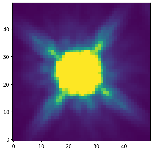
A Point Spread Function (PSF) describes how light from a point source is distributed on detector due to optical effects such as diffraction. Images or cutouts of stars are good approximations of PSFs because stars are single-point sources and their images describe how their light is distributed on the detector. To make cutouts of stars in an image, use the astropy.nddata.Cutout2D function.

The following PSF is a cutout of a star in the Hubble Frontier Fields image of Abell 2744 (same dataset as the example image). Since we will be using the PSF image as a convolution kernel, it is very important that the following requirements are satisfied:

• The image of the PSF should be at the same resolution as the data.

• The star or PSF is centered in the image.

• The PSF image does not contain other sources.

• The image is normalized so that the sum of the PSF image near or equal to 1.0.

• The PSF image should have odd dimensions on each side (because it is a convolution kernel).

from astropy.io import fits

# Load PSF image (2D array)
PSF = fits.getdata('data/f105w_psf.fits.gz')

# Normalize PSF
PSF = PSF / PSF.sum()

# Note that the PSF shape is odd on all sides
print("PSF Shape = {}".format(PSF.shape))

# Plot PSF and use vmax and vmin to show difraction spikes
plt.imshow(PSF, vmin=0, vmax=PSF.std()/10)
plt.show()

PSF Shape = (50, 50)

Sérsic Model

Sérsic Parameters

The amplitude, r_eff, n, x_0, y_0, ellip, and theta represent the galaxy’s brightness, effective radius, Sersic index, position, ellipticity, and orientation, respectively. Here we make rough estimates of the parameters:

amplitude=0.2
r_eff=20
n=1
x_0=107
y_0=70
ellip=0.1
theta=0.1

AstroPy Sérsic Model

Here, we are setting up a 2D galaxy light profile model using astropy’s Sersic2D model. The Sersic2D model is a widely-used representation of the light distribution of elliptical galaxies. We also define a set of bounds, a dictionary of lower and upper bounds of parameters. Keys are parameter names. The values are a list or a tuple of length 2 giving the desired range for the parameter and a value of None means no bounds. The default bounds can be provided using the PetroFit get_default_sersic_bounds function. For example, we restrain the fitter from exploring half-light radii that are negative by adding 'r_eff': (0, None). We also apply a custom restriction for the center of the model to be within a range (center_slack) from the initial guess.

from astropy.modeling import models

center_slack = 20

sersic_model = models.Sersic2D(

        amplitude=amplitude,
        r_eff=r_eff,
        n=n,
        x_0=x_0,
        y_0=y_0,
        ellip=ellip,
        theta=theta,
        bounds = pf.get_default_sersic_bounds({
            'x_0': (x_0 - center_slack/2, x_0 + center_slack/2),
            'y_0': (y_0 - center_slack/2, y_0 + center_slack/2),
        }),
)

sersic_model

<Sersic2D(amplitude=0.2, r_eff=20., n=1., x_0=107., y_0=70., ellip=0.1, theta=0.1)>

PSFConvolvedModel2D

The petrofit PSFConvolvedModel2D is a Fittable2DModel that adds PSF convolution and model to image sampling to astropy core models. PSFConvolvedModel2D makes an image of the underlying model and samples it onto a grid. The model image is then convolved with a PSF if one is provided. Since PSFConvolvedModel2D is a Fittable2DModel, it can be used to fit model images to data images. For example, we wrap an astropy Sersic2D model in this doc with PSFConvolvedModel2D, which produces an oversampled and PSF convolved version of the Sérsic profile at each iteration of the fitting algorithm. Note that ``PSFModel`` is deprecated and replaced by ``PSFConvolvedModel2D``.

Note

PSFConvolvedModel2D is agnostic to the models it wraps and can handle complex multi-component astropy models.

Pixel Centering in PSFConvolvedModel2D

PSFConvolvedModel2D adopts the DS9 coordinate system, where the pixel index corresponds to its center. Thus, an index of 0 designates the center of the first pixel. This is distinct from the GALFIT convention, and users should note this difference when comparing results between tools.

Oversampling

One of the advantages of using PSFConvolvedModel2D is its ability to sample models onto model images. Sometimes the models have regions that have to be oversampled to produce better estimates of the data. PSFConvolvedModel2D can oversample the entire model image or a specific pixel region of the image. The oversampling factor and region can be specified in the oversample keyword argument when wrapping an astropy model or during run time by setting the PSFConvolvedModel2D.oversample attribute.

Disable Oversampling (Defailt)

To disable oversampling, set the oversampling argument or attribute to None

# Disable Oversampling
oversample = None

Oversample Entire Model Image

To oversample the image by a factor, you can pass a single integer value. For example:

# Oversample the entire image by a factor of 4
oversample = 4

Oversample a Fixed Region

To oversample a fixed region of finite size, specify the center pixel, the length of the square region and thee oversampling factor. This means passing a tuple of (center_x, center_y, box_length, oversample_factor). For example:

# Replace the pixel values in a box of
# length 20 cented at (x=50, y=60) with a box of
# the same size that has been oversampled by a factor of 5
# i.e (x=50 y=60, box_length=20, oversample_factor=5)

oversample = (50, 60, 20, 5)

Oversample a Moving Region

If the model is being fit, the center of the model is likely to move around. To account for this, we can specify the names of the model parameters that define the center of the box that we are interested in oversampling as strings. This means passing a tuple of (model_param_x, model_param_y, box_length, oversample_factor). For example:

# Replace the pixel values in a box of
# length 20 cented at (x=model.x_0, y=model.y_0) with a box of
# the same size that has been oversampled by a factor of 5
# i.e (model.x_0, model.y_0, box_length=20, oversample_factor=5)

oversample = ('x_0', 'y_0', 20, 5)

Oversampled PSF

The PSF can have intricate details and variations that are not well-captured if we simply sample at the same rate as the data image. This is where the concept of an oversampled PSF comes into play. An oversampled PSF is essentially a higher-resolution representation of the PSF, capturing its subtle variations with more detail. This is beneficial because, during convolution, these details interact with the underlying data, ensuring a more accurate representation of the light distribution. PSFConvolvedModel2D facilitates this by allowing users to specify an oversampled PSF alongside the model. The psf_oversample keyword argument, or attribute, controls the oversampling factor of the PSF. It’s essential to remember that when working with both oversampled models and PSFs, compatibility is key. The PSFConvolvedModel2D class ensures that the model’s oversampling rate (oversample) is always an integer multiple of the PSF’s oversampling rate (psf_oversample).

# The star image PSF is at the
# same resolution as the data
psf_oversample = 1

Create PetroFit Model

Now that we have an astropy model, PSF and oversampling rule, we can create a PSFConvolvedModel2D model as follows:

psf_sersic_model = pf.PSFConvolvedModel2D(sersic_model, psf=PSF, oversample=4, psf_oversample=1)

The PSFConvolvedModel2D etherates all of the parameters, fixed-parameter rules and parameter bounds from the input astropy model. Notice that a new parameter, psf_pa is added to enable PSF rotation.

print(psf_sersic_model.param_names)

('amplitude', 'r_eff', 'n', 'x_0', 'y_0', 'ellip', 'theta', 'psf_pa')

print(psf_sersic_model.bounds)

{'amplitude': (0.0, None), 'r_eff': (0.001, None), 'n': (0.1, 10.0), 'x_0': (97.0, 117.0), 'y_0': (60.0, 80.0), 'ellip': (0.0, 0.99), 'theta': (-6.283185307179586, 6.283185307179586), 'psf_pa': (None, None)}

PSF Rotation

PSFConvolvedModel2D can to rotate the PSF image until an optimal rotation angle is found. This is useful for when the PSF comes from a dataset where the orientation of the diffraction spikes are not the same as the image being fit. psf_pa is in degrees.

To restrict the bounds of the rotation or disable the PSF rotation, you can set the psf_pa to fixed:

# Limit PSF rotation to -5 to 5 degrees
psf_sersic_model.bounds['psf_pa'] = (-5, 5)

# To disable the PSF rotation,
# you can set the psf_pa to fixed.
psf_sersic_model.fixed['psf_pa'] = True

Accessing the Underlying Model

At any point, a copy of the input model with the same parameter values as the corresponding PSFConvolvedModel2D can be accessed using the PSFConvolvedModel2D.model attribute:

psf_sersic_model.model

<Sersic2D(amplitude=0.2, r_eff=20., n=1., x_0=107., y_0=70., ellip=0.1, theta=0.1)>

Visualize Inital Guess Model

Here we visualize the inital guess model using the plot_fit function:

pf.plot_fit(psf_sersic_model, image.data, vmax=vmax, vmin=vmin, figsize=[3*6, 6])
plt.show()

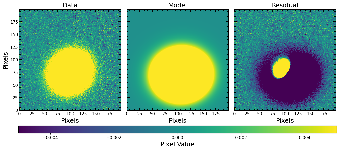
Looks like we better fit this model to optimize its paramters…

Fitting Models

PetroFit uses the Levenberg-Marquardt, Trust Region Reflective algorithm, and linear least-squares algorithms to fit parametrized models. To achieve this, it uses astropy fitting and provides wrappers to fit models to images. One such function is fit_model, which takes any Fittable2DModel model and an image to fit, and returns a fitted copy of the model and the fit_info dictionary. If the image to be fit contains pixels that are set to np.nan, those pixels are ignored by the fitter. The fit_model function also allows us to define parameters, such as maxiter, for the astropy fitter.

Before we fit the image, we compute the weights of each pixel using rms data as follows (please note that weights are optional and set to None by defualt):

fitting_weights = 1 / rms

To fit the galaxy we prepared with the PSFConvolvedModel2D we constructed, we call the fit_model as follows:

%%time

fitted_model, fit_info = pf.fit_model(
    image.data, psf_sersic_model,
    weights=fitting_weights,
    calc_uncertainties=True,
    maxiter=10000,
    epsilon=1.4901161193847656e-08,
    acc=1e-09,
)

CPU times: user 3.45 s, sys: 2.44 s, total: 5.88 s
Wall time: 3.83 s

That’s it! The retuned fitted_model is a copy of the input model (psf_sersic_model) but with the optimized parameter values. We can inspect the parameters of any astropy model using the print_model_params:

pf.print_model_params(fitted_model)

0.2411  amplitude
14.9961 r_eff
0.9993  n
99.9992 x_0
74.9994 y_0
0.1001  ellip
0.7834  theta
0.0000  psf_pa

Paramter Errors

When calc_uncertainties is enabled in the fit_model function, Astropy’s fitter calculates the parameter uncertainties using the covariance matrix. To extract the standard deviation of the parameters, given that the covariance matrix is available:

# covariance matrix dict:
fitted_model.cov_matrix

parameter variances / covariances
amplitude| 0.
r_eff    | -0.,  0.
n        | -0.,  0.,  0.
x_0      | 0., 0., 0., 0.
y_0      |  0., -0.,  0.,  0.,  0.
ellip    | -0.,  0.,  0.,  0.,  0.,  0.
theta    | -0., -0., -0., -0.,  0., -0.,  0.

param_stds = fitted_model.stds
for param, std in zip(param_stds.param_names, param_stds.stds):
    print("{:<10} {}".format(param, std))

amplitude  0.00017220394307486002
r_eff      0.006653704513228788
n          0.0007095453133960075
x_0        0.00245866411273507
y_0        0.0024587921446553767
ellip      0.0004006408007567499
theta      0.00211484907786129

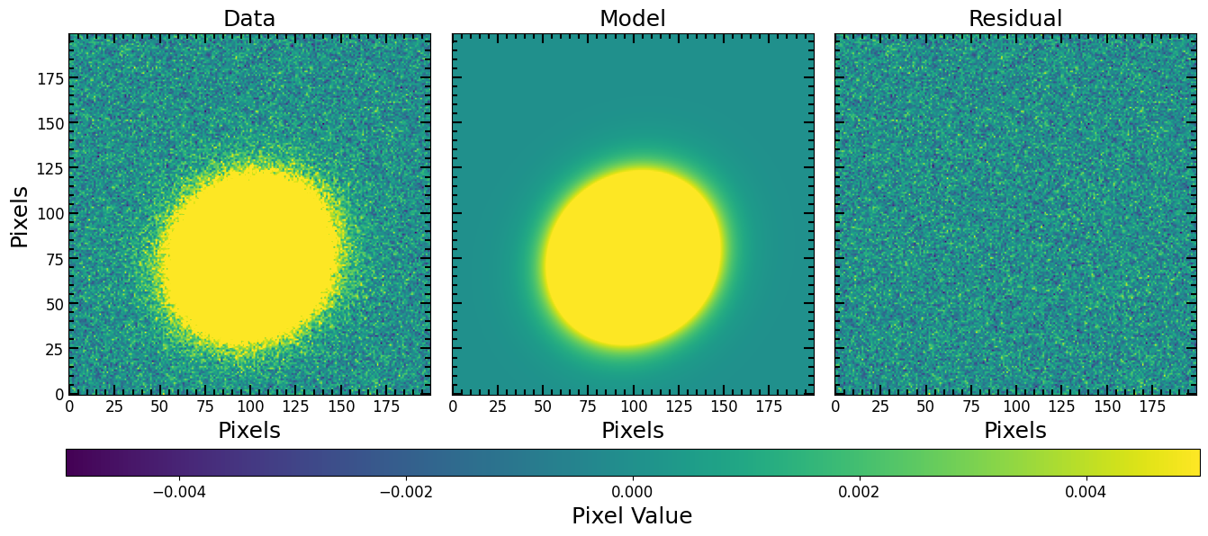
Generate Model Image

To generate a model image we use the plot_fit function. The function, given a 2D model and fitted image, converts the model into a model-image we can visualize and manipulate.

pf.plot_fit(fitted_model, image.data, vmax=vmax, vmin=vmin, figsize=[3*6, 6])
plt.show()