Multi-object Photometry

In this section we demonstrate how to perform photometry on multiple objects in an image. We choose a faint group of galaxies and run the photometry steps as described in the Photometry section.

To start with PetroFit, simply import it as follows:

import petrofit as pf

Loading Example Data

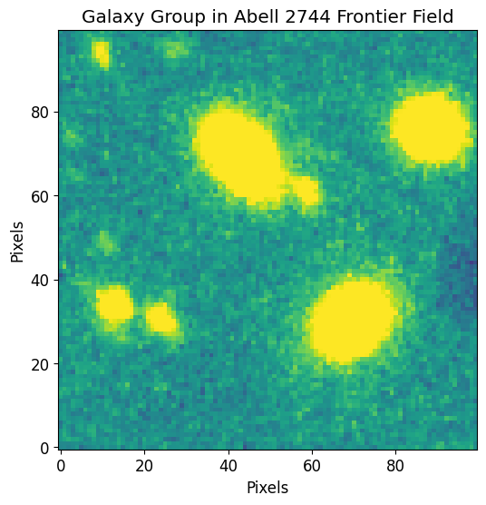
The following data is a cutout of a group of faint galaxies in Abell 2744. The original data was acquired by the Hubble Frontier Fields team via the WFC3 instrument in the F105W filter and can be directly downloaded from the Mikulski Archive for Space Telescopes.

We first use astropy’s CCDData to load the example data and visualize it through matplotlib.

from astropy.nddata import CCDData

image = CCDData.read('data/abell_2744_group_of_galaxies_f105w.fits.gz')

from matplotlib import pyplot as plt

plt.rcParams['figure.figsize'] = [6, 6]
plt.rcParams['image.origin'] = 'lower'
plt.rcParams['font.size'] = 12

vmax =  0.01 # Use the image std as max and min of all plots
vmin = - vmax

plt.imshow(image.data, vmin=vmin, vmax=vmax)
plt.title("Galaxy Group in Abell 2744 Frontier Field")
plt.xlabel("Pixels")
plt.ylabel("Pixels")
plt.show()

Make Source Catalog

We will use the sigma clipped std as a threshold at the segmentation and deblending steps.

from astropy.stats import sigma_clipped_stats

# Compute stats for threshold
image_mean, image_median, image_stddev = sigma_clipped_stats(image.data, sigma=3)

# Define threshold
threshold = image_stddev

# Min Source size (area)
npixels = 5**2


cat, segm, segm_deblend = pf.make_catalog(
    image.data,
    threshold=threshold,
    wcs=image.wcs,
    deblend=True,
    npixels=npixels,
    contrast=0.00,
    plot=True, vmax=vmax, vmin=vmin,
    figsize=[12, 6]
)

plt.show()

# Display source properties
print("Num of Targets:", len(cat))

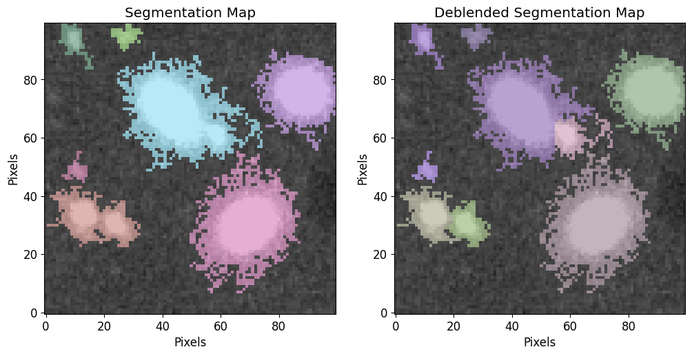
Num of Targets: 9

Photometry Loop

We define the list of aperture radii and proceed to the photometry step. In this case, instead of selecting a source, we loop through the source catalog and perform photometry on each object. After constructing the photometry we create a Petrosian object for the source. We save the Petrosian in a python dictionary (petrosian_properties) for later use.

max_pix=35

r_list = pf.make_radius_list(
    max_pix=max_pix, # Max pixel to go up to
    n=max_pix # the number of radii to produce
)


petrosian_properties = {}

for idx, source in enumerate(cat):

    # Photomerty
    flux_arr, area_arr, error_arr = pf.source_photometry(

        # Inputs
        source, # Source (`photutils.segmentation.catalog.SourceCatalog`)
        image.data, # Image as 2D array
        segm_deblend, # Deblended segmentation map of image
        r_list, # list of aperture radii

        # Options
        cutout_size=max(r_list)*2, # Cutout out size, set to double the max radius
        bg_sub=True, # Subtract background
        sigma=3, sigma_type='clip', # Fit a 2D plane to pixels within 3 sigma of the mean
        plot=False, vmax=vmax, vmin=vmin, # Show plot with max and min defined above
    )
    plt.show()

    p = pf.Petrosian(r_list, area_arr, flux_arr)

    petrosian_properties[source] = p

print("Completed for {} Sources".format(len(petrosian_properties)))

Completed for 9 Sources

Compute Total Mags

We compute the total magnitudes of the sources by looping through their Petrosian objects. We use the flux_to_abmag function to convert the total flux to AB mags of each object.

import numpy as np

mag_list = []

for source in petrosian_properties:

    # Get Petrosian
    p = petrosian_properties[source]

    # Compute HST Flux -> mags for total_flux
    mag = pf.hst_flux_to_abmag(p.total_flux, image.header)

    # Add to mag list
    mag_list.append(mag)

# Convert mag_list to array
mag_list = np.array(mag_list)

mag_list

array([23.78101354, 28.64431073, 24.01132477, 27.41390818, 28.64179264,
       26.41465787, 25.84712754, 23.55719409, 26.37657836])

Photometry Catalog

We construct and save a photometry catalog with the magnitudes we computed. To construct the table, we first use the SourceCatalog.to_table() function that returns an astropy table. This will include important info about each source. We then add a new column (MAG_F105W) with the total mags we computed.

# Segmentation catalog to astropy table.
photo_cat = cat.to_table()

# Add new column with mags.
photo_cat.add_column(mag_list, index=4, name='MAG_F105W')

# Save to file.
photo_cat.write('temp/example_photo_cat.csv', overwrite=True)

photo_cat

QTable length=9

label	xcentroid	ycentroid	sky_centroid	MAG_F105W	bbox_xmin	bbox_xmax	bbox_ymin	bbox_ymax	area	semimajor_sigma	semiminor_sigma	orientation	eccentricity	min_value	max_value	local_background	segment_flux	segment_fluxerr	kron_flux	kron_fluxerr
			deg,deg						pix2	pix	pix	deg
int64	float64	float64	SkyCoord	float64	int64	int64	int64	int64	float64	float64	float64	float64	float64	float64	float64	float64	float64	float64	float64	float64
1	69.32265836375497	30.238019971715627	3.579223902860569,-30.380187463851975	23.7810135425286	50	87	7	55	1000.0	7.066388328760255	5.579720371665397	54.75734563367578	0.6136036659242836	0.0018545736093074083	0.07670669257640839	0.0	10.244122936739586	nan	10.709215362358297	nan
2	10.737608995340572	48.6121151841155	3.580355742519194,-30.379881269181666	28.644310734022653	6	14	45	55	43.0	2.0965997789103628	1.8762638664800115	73.19191801040047	0.4462507287495157	0.0019008400849997997	0.00620837789028883	0.0	0.15271575504448265	nan	0.395127586728858	nan
3	87.92829837715828	75.63296420231474	3.5788644863585364,-30.37943086630141	24.011324773909678	71	99	56	90	569.0	4.684225490343459	4.371347211905419	-44.65368081791386	0.3593419120981481	0.001854302710853517	0.10125063359737396	0.0	8.084702808177099	nan	8.19241690061656	nan
4	9.815810702861459	93.31562288938129	3.580373573168226,-30.37913621099525	27.413908182788763	5	16	84	99	77.0	3.355176286646171	1.6479017677110668	-61.23856024451831	0.8710738471935022	0.0018753919284790754	0.012467581778764725	0.0	0.3568276413716376	nan	0.46358781728153653	nan
5	27.555493767397174	94.91373210653953	3.5800308569397217,-30.37910956468503	28.641792635176103	23	33	90	99	54.0	2.252178183265229	1.8456062428385482	9.760103655188653	0.5731133274324416	0.0018675385508686304	0.006537159439176321	0.0	0.18736975535284728	nan	0.21081410418602697	nan
6	24.481221829558184	30.35265489108243	3.5800902145053146,-30.38018558504191	26.414657874624123	18	32	23	38	137.0	3.1297440100684626	2.368327034962023	-54.918957106073215	0.6537438768702845	0.0018714345060288906	0.02676144801080227	0.0	0.9589369829045609	nan	1.161363705896545	nan
7	12.418600181421457	33.41806848906761	3.5803232591739147,-30.380134502367362	25.84712753793599	1	22	23	43	221.0	4.158127754208604	3.041444861227075	-54.91674752060506	0.6818996401383097	0.0018537540454417467	0.02450975775718689	0.0	1.475870828377083	nan	1.9072046957775326	nan
8	43.420003300978024	69.4761061324968	3.57972435145291,-30.379533514551756	23.557194090925286	25	68	49	89	878.0	6.259160655628094	4.972810345866363	-47.74028219223737	0.607283547825944	0.0018594693392515182	0.13125701248645782	0.0	12.524548709043302	nan	12.935097062743418	nan
9	59.890633529332646	60.66274815897566	3.5794061443723244,-30.379680392014183	26.376578364563656	55	74	53	68	144.0	3.985926639607556	2.811090552294893	0.7501050272960306	0.7089547587670784	0.001866802922450006	0.02579653263092041	0.0	0.9505528409499675	nan	1.816363676057363	nan

Simultaneous Fitting

In this section, we explore how to make compound models that can be used to describe multiple objects in an image. We use the same dataset as the Multi-object Photometry section to fit the nine faint sources with Sersic profiles.

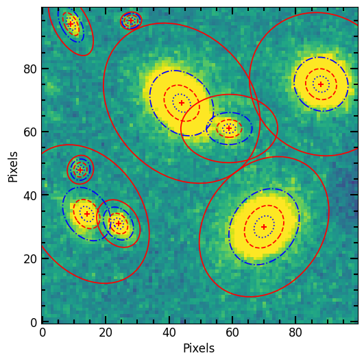
Make Individual Models

To do this we loop through the sources and construct astropy Sersic2D models for each source. We also make initial guesses of the paramters as described in the Estimating Sersic Parameters section. At the end of each iteration, we add the newly constructed model in a list model_list.

from photutils.isophote import EllipseGeometry, Ellipse
from astropy.modeling import models

# AstroPy Model List
model_list = []

# For each source
for source in list(petrosian_properties.keys()):

    # Get Petrosian
    p = petrosian_properties[source]

    # Estimate center
    position = pf.get_source_position(source)
    x_0, y_0 = position

    # Estimate shape
    elong = pf.get_source_elong(source)
    ellip = pf.get_source_ellip(source)
    theta = pf.get_source_theta(source)

    # Estimate Sersic index
    n = 1

    # Estimate r_half_light
    r_eff = p.r_half_light

    # Estimate amplitude
    amplitude = pf.get_amplitude_at_r(r_eff, image, x_0, y_0, ellip, theta)

    # Allow for 4 pixel center slack
    center_slack = 4

    # Make astropy model
    sersic_model = models.Sersic2D(

            amplitude=amplitude,
            r_eff=r_eff,
            n=n,
            x_0=x_0,
            y_0=y_0,
            ellip=ellip,
            theta=theta,

            bounds = pf.get_default_sersic_bounds({
                'x_0': (x_0 - center_slack/2, x_0 + center_slack/2),
                'y_0': (y_0 - center_slack/2, y_0 + center_slack/2),
            }),
    )

    # Add to model list
    model_list.append(sersic_model)

    # Over-plot Petrosian radii
    p.imshow(position=position, elong=elong, theta=theta, lw=1.25)

# Plot image of sources
plt.imshow(image.data, vmax=vmax, vmin=vmin)
pf.mpl_tick_frame()
plt.xlabel('Pixels')
plt.ylabel('Pixels')

plt.show()

Make Compound Model

To make a single compound model that represents all the sources of interest, we add up all the models. astropy models can be added like numbers or arrays, so we convert the model list to a numpy array and sum it.

compound_model = np.array(model_list).sum()

compound_model

<CompoundModel(amplitude_0=0.02231892, r_eff_0=7.18243649, n_0=1., x_0_0=70., y_0_0=30., ellip_0=0.21038583, theta_0=0.95569597, amplitude_1=0.00356518, r_eff_1=2.31946389, n_1=1., x_0_1=12., y_0_1=48., ellip_1=0.10509202, theta_1=1.27743996, amplitude_2=0.03006719, r_eff_2=5.04680936, n_2=1., x_0_2=88., y_0_2=75., ellip_2=0.06679403, theta_2=-0.77935375, amplitude_3=0.00509282, r_eff_3=3.97219444, n_3=1., x_0_3=9., y_0_3=94., ellip_3=0.50884793, theta_3=-1.06881451, amplitude_4=0.0044909, r_eff_4=2.15623125, n_4=1., x_0_4=28., y_0_4=95., ellip_4=0.18052388, theta_4=0.17034594, amplitude_5=0.01000131, r_eff_5=3.48929786, n_5=1., x_0_5=24., y_0_5=31., ellip_5=0.24328411, theta_5=-0.95851662, amplitude_6=0.00696394, r_eff_6=5.01960392, n_6=1., x_0_6=14., y_0_6=34., ellip_6=0.26855425, theta_6=-0.95847806, amplitude_7=0.03945622, r_eff_7=6.24384877, n_7=1., x_0_7=44., y_0_7=69., ellip_7=0.20551483, theta_7=-0.83322511, amplitude_8=0.00847777, r_eff_8=3.95179036, n_8=1., x_0_8=59., y_0_8=61., ellip_8=0.29474604, theta_8=0.0130918)>

Make PSFConvolvedModel2D

Now that we have a single model that represents all the sources, we can create a PSFConvolvedModel2D with the appropriate parameters. After we load the PSF, we wrap the compound model and PSF using PSFConvolvedModel2D. We specify an oversampling factor 4 to account for poor CCD sampling.

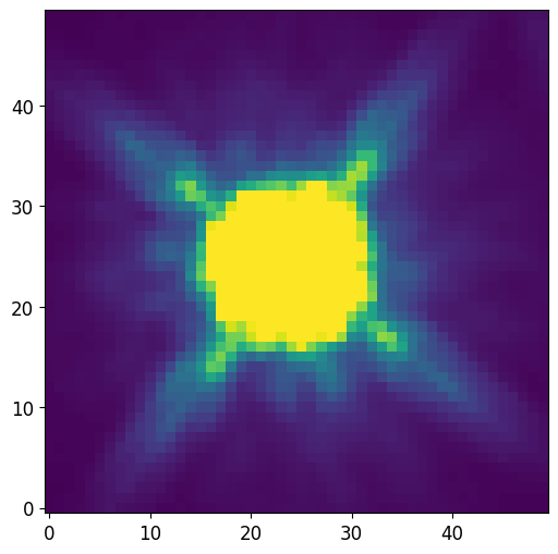
Load and Normalize PSF

from astropy.io import fits

PSF = fits.getdata('data/f105w_psf.fits.gz')
PSF = PSF / PSF.sum()

plt.imshow(PSF, vmin=0, vmax=PSF.std()/10)

<matplotlib.image.AxesImage at 0x7f8035703f90>

PSFConvolvedModel2D

psf_sersic_model = pf.PSFConvolvedModel2D(compound_model, psf=PSF, oversample=4)

psf_sersic_model.fixed['psf_pa'] = True

Fit Model to Data

We fit the compound model using a Levenberg-Marquardt algorithm and save the returned optimized copy of the fitted model in fitted_model. Since this the compound model is composed of many parameters, we may see astropy warnings when the fitter explores parameters that cause issues, such as division by zero.

%%time

fitted_model, _ = pf.fit_model(
    image.data, psf_sersic_model,
    maxiter=10000,
    epsilon=1.4901161193847656e-08,
    acc=1e-09,
)

CPU times: user 2min 26s, sys: 7.98 s, total: 2min 34s
Wall time: 2min 22s

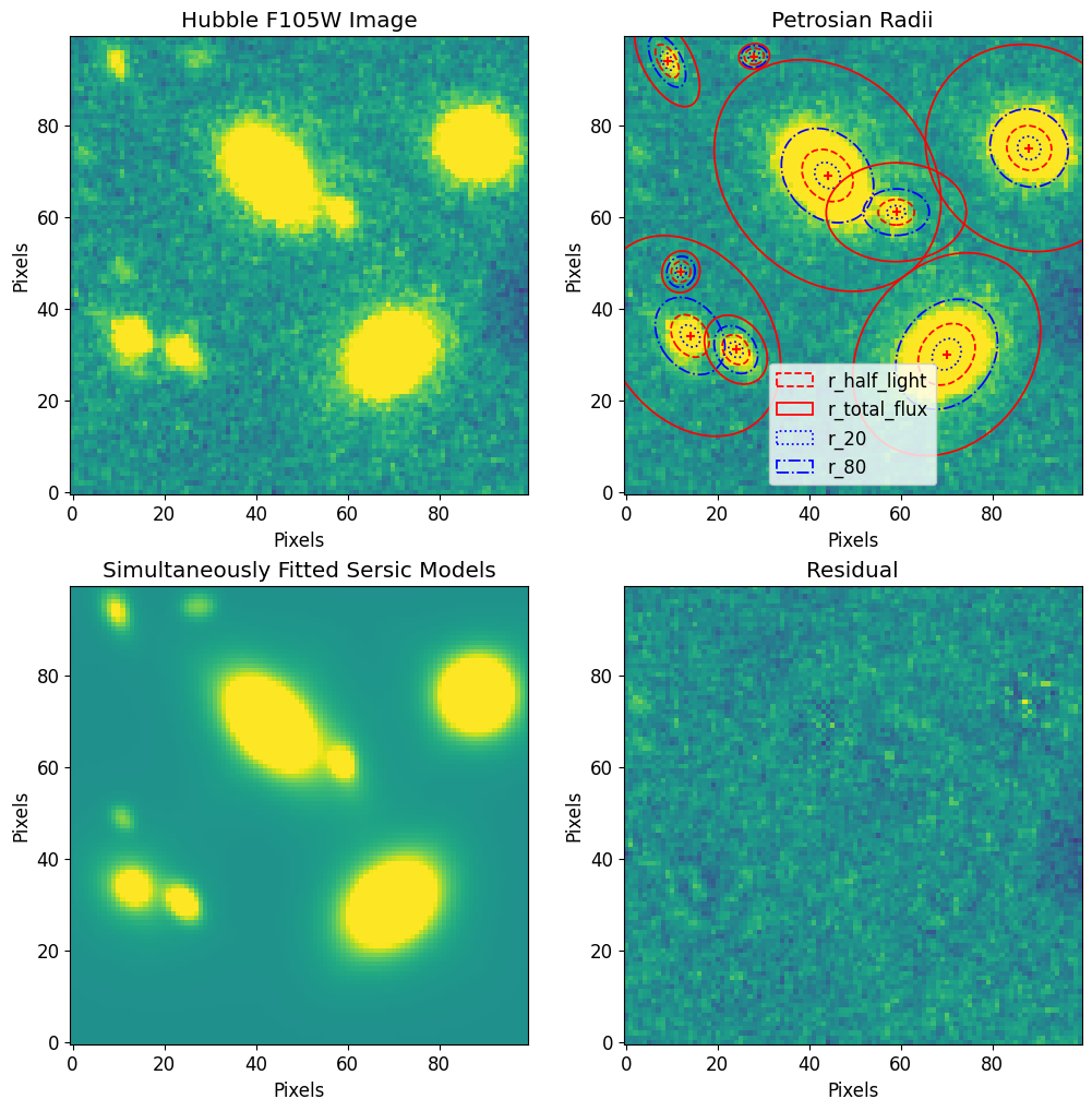
Generate Model Image

To generate a model image we use the model_to_image utility function. This function allows us to define the center of the model image and the side length of the image.

# Make Model Image
# ----------------

# Set the size of the model image equal to the original image
full_fitted_image_size = image.data.shape[0]

# Center the model image at the center of the original image
# so the two images cover the same window
full_fitted_image_center = full_fitted_image_size // 2

# Generate a model image from the model
fitted_model_image = pf.model_to_image(
    fitted_model,
    full_fitted_image_size,
)

# Plot Model Image
# ----------------

fig, ax = plt.subplots(2, 2, figsize=[12, 12])

# Plot raw data
im = ax[0, 0].imshow(image.data, vmin=vmin, vmax=vmax)
ax[0, 0].set_title("Hubble F105W Image")
ax[0, 0].set_xlabel("Pixels")
ax[0, 0].set_ylabel("Pixels")
#ax[0, 0].axis('off')

# Plot Petrosian radii
plt.sca(ax[0, 1])
for i, source in enumerate(petrosian_properties):
    p = petrosian_properties[source]

    position = pf.get_source_position(source)
    x_0, y_0 = position

    elong = pf.get_source_elong(source)
    ellip = pf.get_source_ellip(source)
    theta = pf.get_source_theta(source)

    p.imshow(position=position, elong=elong, theta=theta, lw=1.25)
    if i == 0:
        plt.legend()
ax[0, 1].imshow(image.data, vmin=vmin, vmax=vmax)
ax[0, 1].set_title("Petrosian Radii")
ax[0, 1].set_xlabel("Pixels")
ax[0, 1].set_ylabel("Pixels")
# ax[0, 1].axis('off')

# Plot Model Image
ax[1, 0].imshow(fitted_model_image, vmin=vmin, vmax=vmax)
ax[1, 0].set_title("Simultaneously Fitted Sersic Models")
ax[1, 0].set_xlabel("Pixels")
ax[1, 0].set_ylabel("Pixels")
# ax[1, 0].axis('off')

# Plot Residual
ax[1, 1].imshow(image.data - fitted_model_image, vmin=vmin, vmax=vmax)
ax[1, 1].set_title("Residual")
ax[1, 1].set_xlabel("Pixels")
ax[1, 1].set_ylabel("Pixels")
# ax[1, 1].axis('off')

plt.show()

Analysis of Background

We can now create a background image using the residual and perform some statistical analysis on it.

# Define background image
background_image = image.data - fitted_model_image

# Compute stats
# -------------

noise_mean = background_image.mean()
noise_sigma = background_image.std()
noise_3_sigma = noise_sigma * 3.
noise_8_sigma = noise_sigma * 8.

print("noise_mean = {}".format(noise_mean))
print("noise_sigma = {}".format(noise_sigma))
print("noise_3_sigma = {}".format(noise_3_sigma))

# Plots
# -----

fig, axs = plt.subplots(1, 2, figsize=[16, 8])
plt.sca(axs[0])
plt.imshow(image.data - fitted_model_image, vmin=vmin, vmax=vmax)
plt.title('Residual Image')

plt.sca(axs[1])
n, bins, patches = plt.hist(background_image.flatten(), bins=35, align='left',
                            color='black', label="Binned Residual Image Pixel Values")
plt.plot(bins[:-1], n, c='r', linewidth=3)
plt.axvline(image.data.mean(), label="Raw Input Image Mean", c='g',linestyle="--")
plt.axvline(noise_mean, label="Residual Image Mean", linestyle="--")


plt.xlabel('Flux Bins [{}]'.format(str(image.unit)))
plt.ylabel('Count')
plt.title('Residual Image Pixel Value Histogram')
plt.legend()

plt.show()

noise_mean = 5.009439712276197e-05
noise_sigma = 0.0013882674260103844
noise_3_sigma = 0.004164802278031153

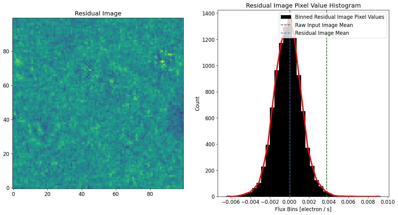
Now we see the residual image mean is near that is near the mean of the noise distribution, we can make a segmentation map using the residual image 3-sigma as the detection threshold. Notice how some of the sources we were able to fit were below the 3-sigma estimate of the background (residual image).

new_threshold = noise_3_sigma

new_cat, new_segm, new_segm_deblend = pf.make_catalog(
    image.data,
    threshold=new_threshold,
    wcs=image.wcs,
    deblend=True,
    npixels=npixels,
    contrast=0.00,
    plot=True, vmax=vmax, vmin=vmin,
    figsize=[12, 6]
)

plt.show()

# Display source properties
print("Num of Targets:", len(new_cat))

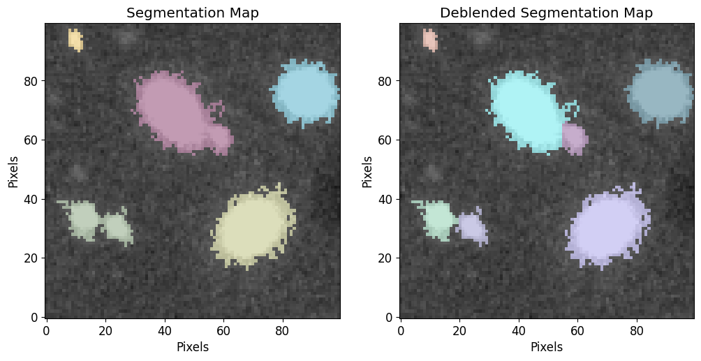
Num of Targets: 7