Photometry

To measure the Petrosian properties of galaxies, we construct a photometric curve of growth using a set of concentric apertures with varying radii to measure the flux. From this curve of growth, we will measure different properties of the galaxy including the total flux, characteristic radii such as the Petrosian radius and half-light radius, and the concentration index in the Petrosian section below. For a quick guide on how to construct curves of growth and Petrosian profiles, please see the Making a Photutils Source Catalog and Curve of Growth and Petrosian Radii sections in the Quick Start guide.

To start with PetroFit, simply import it as follows:

import petrofit as pf

Loading Example Data

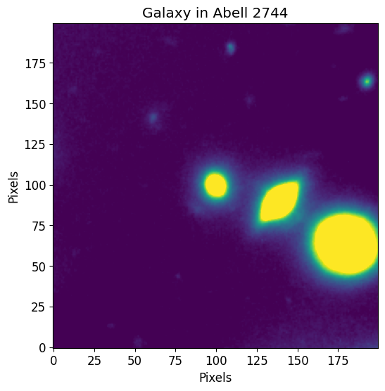
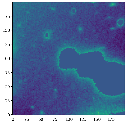
The following data is a cutout of a group of bright galaxies in Abell 2744 (located at (3.596248, -30.388517)). The original data was acquired by the Hubble Frontier Fields team via the WFC3 instrument in the F105W filter and can be directly downloaded from the Mikulski Archive for Space Telescopes. The cutout image used in this documentation can be found in the git repository at the following path petrofit/docs/data/abell_2744_dwarf_galaxy_f105w.fits.gz.

We first use astropy’s CCDData to load the example data and visualize it through matplotlib.

from astropy.nddata import CCDData
from astropy.io import fits

image = CCDData.read('data/abell_2744_dwarf_galaxy_f105w.fits.gz')
rms = fits.getdata('data/abell_2744_dwarf_galaxy_f105w_rms.fits.gz')

from matplotlib import pyplot as plt

plt.rcParams['figure.figsize'] = [6, 6]
plt.rcParams['image.origin'] = 'lower'
plt.rcParams['font.size'] = 12

vmax = image.data.std() # Use the image std as max and min of all plots
vmin = - vmax

plt.imshow(image.data, vmin=0, vmax=image.data.std())
plt.title("Galaxy in Abell 2744")
plt.xlabel("Pixels")
plt.ylabel("Pixels")
plt.show()

Estimate Data Noise at Dark Area

In this section, we estimate the noise levels in the image using astropy’s sigma_clipped_stats and photutils’s calc_total_error functions.

from astropy.stats import sigma_clipped_stats
image_mean, image_median, image_stddev = sigma_clipped_stats(image.data, sigma=3)

from photutils.utils import calc_total_error
err = calc_total_error(
    data=image.data, # Input Image
    bkg_error=rms, # All sources of background error except source Poisson error
    effective_gain=image.header['EXPTIME'] # Factor to convert data units to counts
)

Catalogs

Before we can perform photometry, we need to first identify the sources in the image. To do this, we use Photutils and the wrappers in PetroFit.

Make Catalog

We first start by defining the detection threshold and we select this value to be 3-sigma for this example.

# Define detect threshold
threshold = 3*image_stddev

We also have to define the number of pixels that make up the smallest object. npixels is the number of connected pixels, each greater than the threshold value, that an object must have to be detected. npixels must be a positive integer.

npixels = 4**2

To make a catalog of sources and segmentation maps, we use petrofit’s make_catalog function. The function returns a source catalog (photutils.SourceCatalog), a segmentation image, and, if deblend=True, a deblended segmentation image.

The make_catalog function wraps three steps into one function:

1. Segmentation:

   To identify sources in the image, we first segment the image. The image is smoothed with a gaussian kernel if kernel_size is provided and clipped at the threshold specified (after smoothing if applicable). The image is then segmented using the petrofit.segmentation.make_segments function, which is a wrapper for photutil’s detect_sources functionality.

2. Deblending:

   To further distinguish the sources, we use photutils.deblend_sources to deblend the sources into individual galaxies. The contrast parameter is the fraction of the total (blended) source flux that a local peak must have (at any one of the multi-thresholds) to be considered as a separate object and nlevels is the number of multi-thresholding levels to use. If deblend is set to False, None is returend for segm_deblend.

3. Source Catalog:

   Now that we have deblended the sourecs into individual sources, the next step is to create a source catalog (photutils.SourceCatalog) that contains properties like (xcentroid, ycentroid), eccentricity and area. Note that the deblended map is used to make the source catalog but if deblend is set to False, the segmentation map is used instead.

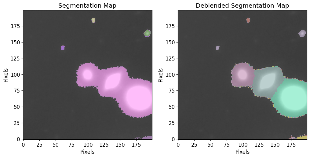
By setting the plot flag to True, we see plots of the segmentation and deblended segmentation maps. The image is plotted along with a color-coded overplot of the segmentation map (each source is a different color). vmax and vmin can be used the same way as in plt.imshow.

After the computation, the following objects are returned:

• cat : A catalog of sources.

• segm : Segmentation map.

• segm_deblend : Deblended segmentation map.

cat, segm, segm_deblend = pf.make_catalog(
    image.data,
    threshold,
    wcs=None,
    deblend=True,
    npixels=npixels,
    nlevels=30,
    contrast=0.001,
    plot=True, vmax=vmax, vmin=vmin,
    figsize=(12, 6)
)

To demonstrate the useful information in the catalog, we convert the SourceCatalog to an astropy.table.Table and display the first 10 objects.

# Display source properties
print("Num of Targets:", len(cat))

# Convert to table
cat_table = cat.to_table()

cat_table[:10]

Num of Targets: 8

QTable length=8

label	xcentroid	ycentroid	sky_centroid	bbox_xmin	bbox_xmax	bbox_ymin	bbox_ymax	area	semimajor_sigma	semiminor_sigma	orientation	eccentricity	min_value	max_value	local_background	segment_flux	segment_fluxerr	kron_flux	kron_fluxerr
								pix2	pix	pix	deg
int64	float64	float64	object	int64	int64	int64	int64	float64	float64	float64	float64	float64	float64	float64	float64	float64	float64	float64	float64
1	61.08347174238899	141.05186559012205	None	59	64	138	144	34.0	1.7994370638925237	1.2826901873829257	72.98283673407356	0.7013382917172669	0.010554540902376175	0.026845833286643028	0.0	0.5834723142907023	nan	1.8317878434947907	nan
2	192.36299560404697	163.40391871827393	None	187	197	158	169	86.0	2.3144983589944554	1.9834471217713212	53.65520486998864	0.5153724293039628	0.010591089725494385	0.0929785966873169	0.0	2.8758262349292636	nan	3.2707537413335355	nan
3	108.72693550508657	183.8851479597333	None	106	111	180	187	37.0	1.8003927404449662	1.257057560548163	-87.14736406479223	0.7158901102937193	0.010464809834957123	0.045437149703502655	0.0	0.8372195269912481	nan	1.0690440471675258	nan
4	176.59884904430535	1.7105077906435575	None	172	181	0	5	22.0	2.5652493504083584	1.2345618770639404	13.128240218386493	0.876575763829376	0.010684505105018616	0.01434874627739191	0.0	0.26085690688341856	nan	3.44449120866383	nan
5	192.09296727764394	1.82553577948899	None	180	199	0	7	84.0	4.976606287872485	1.5422939287464803	5.980651162675711	0.9507662987626069	0.010602000169456005	0.02371048368513584	0.0	1.247399945743382	nan	3.590573711610179	nan
6	178.73633119059068	63.493826518219336	None	143	199	33	95	2704.0	9.40299866437019	9.177157386885888	-48.66212288913661	0.21785120428951427	0.010437765158712864	3.6771397590637207	0.0	421.7741427142173	nan	422.6815556552462	nan
7	138.55898473281684	89.25004484979968	None	109	166	63	112	1864.0	7.532153967377171	5.563519557842017	44.31309259442659	0.6741045627289916	0.010432953014969826	3.6545557975769043	0.0	244.33296140562743	nan	240.57513423073874	nan
8	99.92859014542458	99.15188824983441	None	83	118	80	118	1114.0	6.7507255757709	6.379388610260266	76.6082699457646	0.32709046915385503	0.010427203960716724	0.44580602645874023	0.0	56.775723142549396	nan	60.32600669722427	nan

Plotting Segmentation Maps

To plot segmentations, you can use the plot_segments function included in PetroFit as follows:

pf.plot_segments(segm, image=image.data, vmax=vmax, vmin=vmin)

As you can see, the segmentation resulted in the identification sources but the sources at the center were classified as a single object because they have interconnecting pixels that are above the threshold.

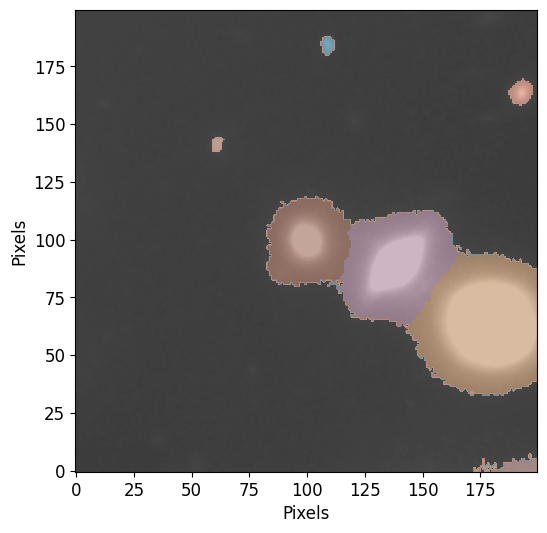
Next we use the same functiton to plot the deblended segmentation map, notice how the central sources are now deblended into individual sources:

pf.plot_segments(segm_deblend, image=image.data, vmax=vmax, vmin=vmin)

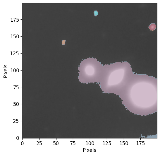
We can also plot the background pixels that are not a part of a source’s segmentation footprint using the plot_segment_residual function. We significantly lower the vmax and vmin values so the background pixels become more apparent. This plot can be used to see if the threshold used to segment the image was too high. If the threshold is high, we would notice bright pixels that are part of the source in this plot.

pf.plot_segment_residual(segm, image.data, vmax=vmax/5)

Photometry on Single Source

The purpose of this step is to perform aperture photometry to construct a curve of growth that we can use for the Petrosian measurements.

Source Selection

For this example, we will focus on a single source. We have included a helper function order_cat that will produce a list of indices sorted by a key (default is ‘area’). We use the order_cat function to identify the source of interest and perform photometry on its cutout.

# Sort and get the largest object in the catalog
sorted_idx_list = pf.order_cat(cat, key='area', reverse=True)
idx = sorted_idx_list[1] # index 0 is largest
source = cat[idx]  # get source from the catalog

Aperture Radii

To construct the curve of growth, we measure the photometry using circular and/or elliptical apertures of varying, concentric radii that are centered on the source. Before we perform the photometry, we need to provide a list of radii that will be used to construct the circular and elliptical apertures. To achieve this, we have provided a helper function that takes in the max radius in pixels (max_pix) and the number radii (n). The function will return a list of radii by dividing the range (max_pix/n, max_pix) into n equally spaced integers.

r_list = pf.make_radius_list(
    max_pix=50, # Max pixel to go up to
    n=50 # the number of radii to produce
)

print(repr(r_list))

array([ 1.,  2.,  3.,  4.,  5.,  6.,  7.,  8.,  9., 10., 11., 12., 13.,
       14., 15., 16., 17., 18., 19., 20., 21., 22., 23., 24., 25., 26.,
       27., 28., 29., 30., 31., 32., 33., 34., 35., 36., 37., 38., 39.,
       40., 41., 42., 43., 44., 45., 46., 47., 48., 49., 50.])

Photometry Calculation

The source_photometry function is used to perform photometry on a single source (photutils.segmentation.catalog.SourceCatalog). In this example, we provide the function with the source object, the raw image (note that this is the 2D array and not CCDData), segmentation from the last step (SegmentationImage) and the list of radii we made using make_radius_list. Given these parameters and the options below the function performs photometry as follows:

• The positions (max value of source in pixels), elongation and position-angle of the source are determined from the SourceCatalog object. The position will be used to center the apertures and the elongation and position angles will be used as parameters of the elliptical apertures. Each of the radii will be assigned an elliptical aperture with these parameters.

• If cutout_size is defined, the code will use it to make a cutout of that size with the source centered. If the cutout_size is larger than the image or contains pixels outside the image, those pixels outside of the image are replaced by np.nan.

• Once the cutout_size is determined, cutouts of the error map (if provided) and image are produced. Before the raw image is cutout, sources that are not the source of interest are masked using the segmentation map. The mask_background option gives us the ability to also mask pixels that are considered to be background pixels because they do not belong to any source’s segmentation map. All masked pixels are replaced by np.nan and are not counted in the returned area array.

• If bg_sub is set to true, a 2D plane is used to fit pixels that are below a specified sigma from the mean using the petrofit.fitting.fit_plane function. The sigma sigma value is used to determine noise pixels. Once the pixels above this value are masked, a 2D plane is fit to determine the background. The 2D plane model is then converted into an image and subtracted from the cutout of the target source. sigma_type is used to set how this sigma value will be used. The sigma_type options are 'clip' and 'bound':

  • 'clip' (default): Uses astropy.stats.sigma_clipping.sigma_clip to clip at the provided sigma std value. Note that sigma in this case is the number of stds above the mean.

  • 'bound' : After computing the mean of the image, clip at mean - sigma and mean + sigma. Note that sigma in this case is a value and not the number of stds above the mean.

• The resulting image (after being noise subtracted if bg_sub is set to true) is passed to the petrofit.photometry.photometry_step which constructs the apertures and performs photometry.

After calculating the photometry at each radius, three arrays are returned:

• flux_arr: Photometric sum in aperture.

• area_arr: Exact area of the aperture.

• error_arr: if error map is provided, error of measurements.

# Photomerty
flux_arr, area_arr, error_arr = pf.source_photometry(

    # Inputs
    source, # Source (`photutils.segmentation.catalog.SourceCatalog`)
    image.data, # Image as 2D array
    segm_deblend, # Deblended segmentation map of image
    r_list, # list of aperture radii
    error=err,

    # Options
    cutout_size=max(r_list)*2, # Cutout out size, set to double the max radius
    bg_sub=True, # Subtract background
    sigma=3, sigma_type='clip', # Fit a 2D plane to pixels within 3 sigma of the mean
    plot=True, vmax=vmax, vmin=vmin, # Show plot with max and min defined above
)
plt.show()

7

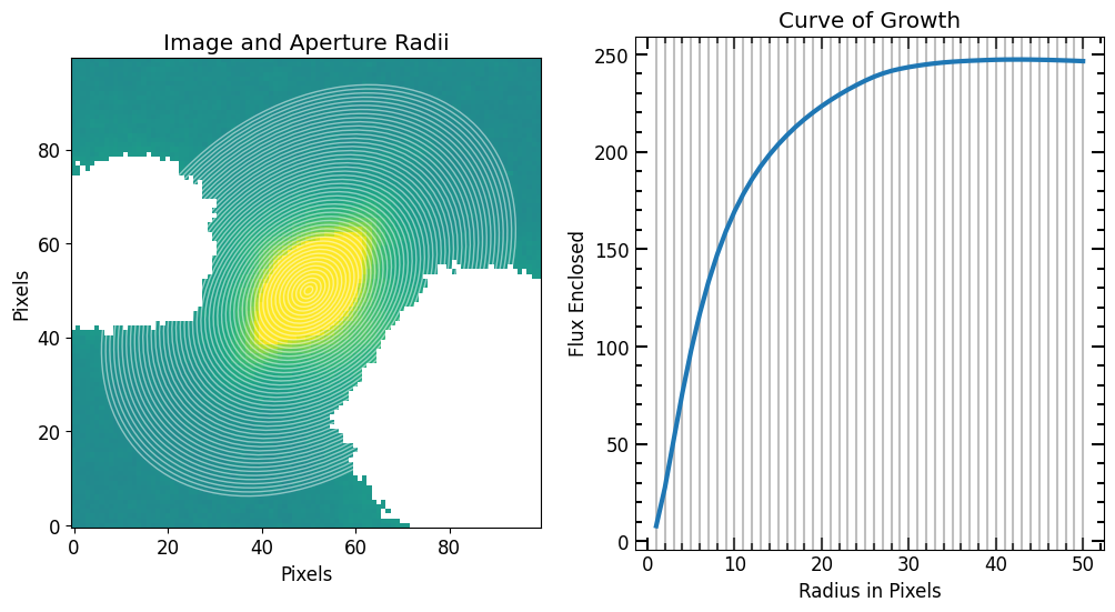
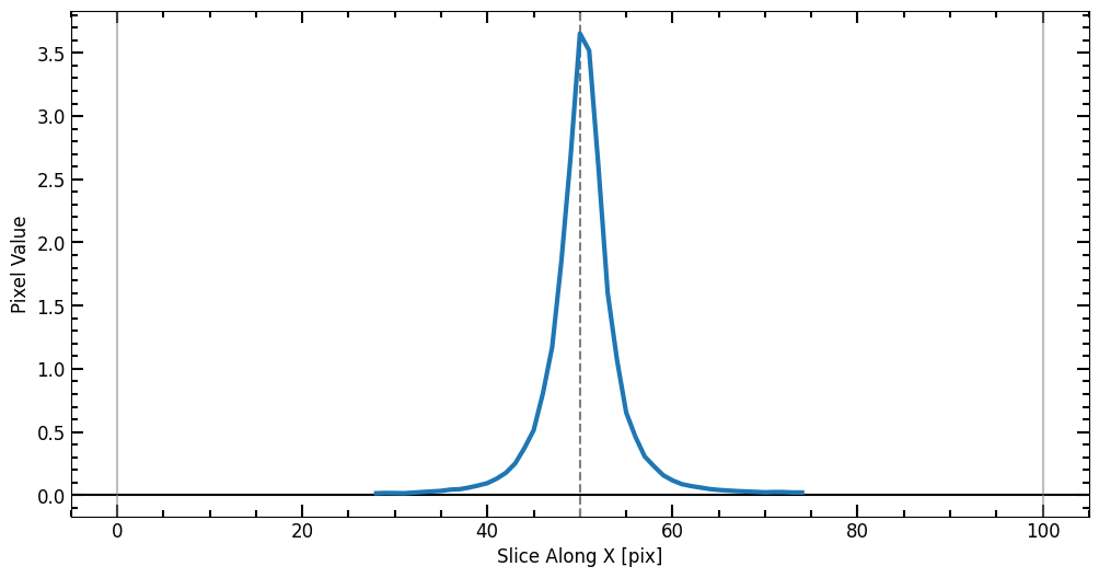
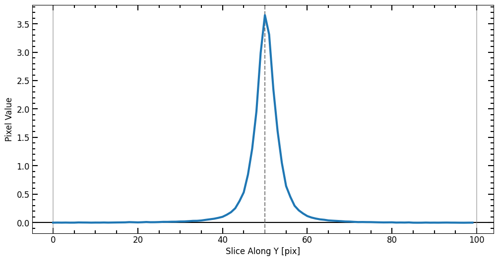
If source_photometry’s plot option is set to True, four plots are displayed: - The top left plot shows the cutout with the 2D plane background subtraction and the surrounding sources masked (replaced by np.nan). - The top right plot shows the curve of growth with increasing radius. The red lines represent the aperture radius. - The bottom two plots show the source profile sliced at the center of the image in the y and x direction respectively.

Save Photometry Arrays

There are many ways of saving the photometry results. For example adding the photometry to the source catalog with the radii as columns. One simple way to save the results for a single source is to save it as a csv of ecsv file using AstroPy Table.

from astropy.table import Table

t = Table(
    data=[r_list, flux_arr, area_arr, error_arr],
    names=['r_list', 'flux_arr', 'area_arr', 'error_arr'],
)


t[:10] # Show first 10 radii

Table length=10

r_list	flux_arr	area_arr	error_arr
float64	float64	float64	float64
1.0	7.753508	2.320493	0.011168
2.0	27.470488	9.281973	0.021141
3.0	51.868013	20.884439	0.029355
4.0	76.013873	37.127891	0.03601
5.0	97.787811	58.01233	0.041509
6.0	116.781632	83.537756	0.046185
7.0	133.120986	113.704168	0.050296
8.0	147.100726	148.511566	0.054002
9.0	159.118392	187.95995	0.057433
10.0	169.405595	232.049321	0.060678

# also save shape information in the table's meta
t.meta['position'] = pf.get_source_position(source)
t.meta['elong'] = pf.get_source_elong(source)
t.meta['theta'] = pf.get_source_theta(source)

t.write('temp/abell_2744_galaxy_f105w_photometry.ecsv', overwrite=True)

Plot Curve of Growth

Here we plot the curve of growth:

plt.errorbar(r_list, flux_arr, yerr=error_arr,
             marker='o', capsize=3, label="Data")

pf.mpl_tick_frame()

plt.xlabel("Aperture Radius [pix]")
plt.ylabel("$L(\leq r)$")
plt.show()